[PYTHON] An introduction to statistical modeling for data analysis

For my own study. The inside is written in R, so I will rewrite it to Python and do my best. Comment out in the code is R language.

2.1 Example: Statistical modeling of seed numbers

It seems that R has count data for the number of seeds. I think it's better to process using numpy, pandas, so Data is also prepared for each of numpy.array and pandas.Series. Also pyplot for graphs.

>>> data = [2, 2, 4, 6, 4, 5, 2, 3, 1, 2, 0, 4, 3, 3, 3, 3, 4, 2, 7, 2, 4, 3, 3, 3, 4, 3, 7, 5, 3, 1, 7, 6, 4, 6, 5, 2, 4, 7, 2, 2, 6, 2, 4, 5, 4, 5, 1, 3, 2, 3]
>>> import numpy
>>> import pandas
>>> matplotlib.pyplot as plt
>>> ndata = numpy.asarray(data)
>>> pdata = pandas.Series(data)

The number of seeds is 50.

# length(data)
>>> len(data)
50
>>> len(ndata)
50
>>> len(pdata)
50

To display sample mean, minimum value, maximum value, quartile, etc. of data

# summary(data)
>>> pdata.describe()
count    50.00000
mean      3.56000
std       1.72804
min       0.00000
25%       2.00000
50%       3.00000
75%       4.75000
max       7.00000
dtype: float64

Get frequency distribution

# table(data)
>>> pdata.value_counts()
3    12
2    11
4    10
5     5
7     4
6     4
1     3
0     1
dtype: int64

It can be confirmed that the number of seeds is 5 and the number of seeds is 6.

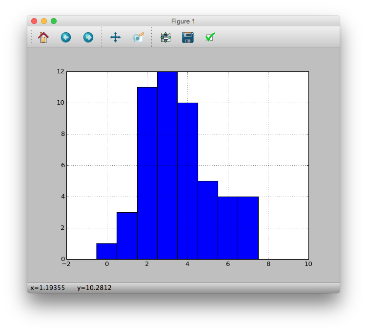
Display this as a histogram

# hist(data, breaks = seq(-0.5, 9.5, 1))
>>> pdata.hist(bins=[i - 0.5 for i in xrange(11)])
<matplotlib.axes._subplots.AxesSubplot object at 0x10f1a9a10>
>>> plt.show()

Calculation of the statistic "sample variance" that represents the variability of data. It seems that the default variance calculation method is different between numpy and pandas. (Reference) By the way, in the case of R, it seems to be an unbiased estimator.

# var(data)
>>> numpy.var(ndata) #Sample statistic
2.9264000000000006
>>> numpy.var(ndata, ddof=True) #Unbiased estimator
2.9861224489795921
>>> pdata.var() #Unbiased estimator
2.986122448979593
>>> pdata.var(ddof=False) #Sample statistic
2.926400000000001

The standard deviation seems to behave in the same way as the variance. This time only the example of pandas.

# sd(data)
>>> pdata.std()
1.7280400600042793

# sqrt(var(data))

2.2 Looking at the correspondence between data and probability distribution

It can be seen that the seed number data has the following characteristics.

--Count data that can be counted as one, two, ... ――The sample average number of seeds per individual is $ 3.56 $ ――There are variations in the purpose of each individual, and if you draw a histogram, it will be a mountain distribution.

The ** probability distribution ** is used to represent the variability. To represent the seed number data as a statistical model This time, it seems that ** Poisson distribution ** is used.

The number of seeds $ y_i $ of a certain plant individual $ i $ is called a ** random variable **.

What is the probability that the number of seeds for individual 1 will be $ y_1 = 2 $?

The probability distribution that expresses is defined by a relatively simple mathematical formula, and its shape is determined by the parameters.

For the Poisson distribution, the only parameter is the ** mean of the distribution **.

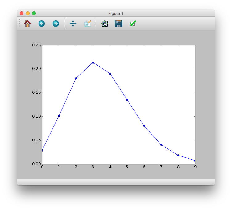
In this example, the Poisson distribution has an average of $ 3.56 $. As for the distribution relationship, scipy seems to be good.

# y <- 0:9
# prob <- dpois(y, lambda = 3.56)
# plot(y, prob, type="b", lyt=2)
>>> import scipy.stats as sct
>>> y = range(10)
>>> prob = sct.poisson.pmf(y, mu=3.56)
>>> plt.plot(y, prob, 'bo-')
>>> plt.show()

Try to overlay with actual data

>>> pdata.hist(bins=[i - 0.5 for i in range(11)])
>>> pandas.Series(prob*50).plot()
>>> plt.plot()

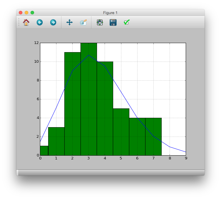
From this result, it is considered that the observation data can be expressed by the Poisson distribution.

2.3 What is the Poisson distribution?

A little more detail about the Poisson distribution.

Definition of Poisson distribution

Random variable when the mean is $ \ lambda $ Probability when the variable is $ y $

p(y|\lambda) = \frac{\lambda ^{y}\exp(-\lambda)}{y!}

nature

-The shape of the curve changes depending on the value of $ \ lambda $ -Take the value of $ y \ in $ {$ 0, 1, 2, \ dots, \ infinty $} and for all $ y $

\sum^{\infty}_{y=0}p(y|\lambda) = 1

--The average of the probability distribution is $ \ lambda $ ($ \ lambda \ geq 0 $) —— Variance and mean are equal

Reasons for choosing the Poisson distribution this time

1. The value $ y_i $ contained in the data is a non-negative integer (count data)
2. $ y_i $ has a lower limit (0) but no upper limit
3. The mean and variance of the observed data are almost equal

2.4 Maximum likelihood estimation of Poisson distribution parameters

Maximum likelihood estimation method

A method of determining the statistic that represents the "goodness of fit" of a model called ** likelihood **.

For Poisson distribution, determine $ \ lambda $.

The product of the probabilities $ p (y_i | \ lambda) $ for all individual $ i $ when a certain $ \ lambda $ is determined

Likelihood is written as $ L (\ lambda) $. In this case,

\begin{eqnarray*}
L( \lambda ) &=& (y_Probability that 1 is 2) \times (y_Probability that 2 is 2) \times \dots \times (y_Probability that 50 is 3)\\
&=& p(y_1 | \lambda) \times p(y_2 | \lambda) \times p(y_3 | \lambda) \times \dots \times p(y_50 | \lambda)\\
&=& \prod_{i}p(y_i | \lambda) = \prod_{i} \frac{\lambda^{y_i} \exp (-\lambda)}{y_i !}
\end{eqnarray*}
 

It becomes. The product is used to calculate the probability that 50 individuals will be the same as the observation (= the probability that 50 events are true).

Since it is difficult to use the likelihood function $ L (\ lambda) $ as it is, the ** log likelihood function ** is generally used.

\begin{eqnarray*}
\log L(\lambda) &=& \log \left( \prod_{i} \frac{\lambda^{y_i} \exp (-\lambda)}{y_i !} \right) \\
&=& \sum_i \log \left( \frac{\lambda^{y_i} \exp (-\lambda)}{y_i !} \right) \\
&=& \sum_i \left( \log(\lambda^{y_i} \exp (-\lambda)) - \log y_i !   \right)\\
&=& \sum_i \left( y_i \log \lambda - \lambda - \sum^{y_i}_{k} \log k \right)
\end{eqnarray*}

Graph the relationship between this log-likelihood $ \ log L (\ lambda) $ and $ \ lambda $.

# logL <- function(m) sum(dpois(data, m, log=TRUE))
# lambda <- seq(2, 5, 0.1)
# plot(lambda, sapply(lambda, logL), type="l")
>>> logL = lambda m: sum(sct.poisson.logpmf(data, m))
>>> lmd = [i / 10. for i in range(20, 50)]
>>> plt.plot(lmd, [logL(m) for m in lmd])
>>> plt.show()

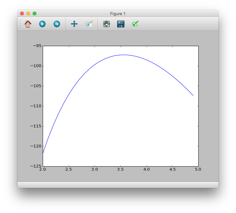
Since the log-likelihood $ \ log L (\ lambda) $ is a monotonically increasing function of the likelihood $ L (\ lambda) $, When the log-likelihood is maximum, the likelihood is also maximum.

Looking at the graph, you can see that the highest probability is around $ \ lambda = 3.5 $.

The specific maximum value may be the maximum value of the log-likelihood (= when the slope becomes 0).

In other words

\begin{eqnarray*}
\frac{\partial \log L(\lambda)}{\partial \lambda} = \sum_i \left\{ \frac{y_i}{\lambda} - 1 \right\} = \frac{1}{\lambda} \sum_i y_i - 50 &=& 0 \\
\lambda &=& \frac{1}{50}\sum_i y_i \\
&=& \frac{All y_i sum}{The number of data}(=Sample mean of data) \\
&=& 3.56
\end{eqnarray*}

The $ lambda $ that maximizes the log-likelihood and likelihood is called the ** maximum likelihood estimate **, and the $ \ lambda $ evaluated by specific $ y_i $ is called the ** maximum likelihood estimate **. ..

Generalization

Let $ p (y_i | \ theta) $ be the probability that the observed data $ y_i $ is generated from the probability distribution with $ \ theta $ as a parameter. Likelihood, log-likelihood

\begin{eqnarray*}
L(\theta | Y) &=& \prod_i p(y_i | \theta) \\

\log L(\theta | Y) &=& \sum_i \log p(y_i | \theta)

\end{eqnarray*}

It becomes.

How to choose a probability distribution

Consider the following points.

――Is the quantity you want to explain discrete or continuous? ――What is the range of the amount you want to explain? ――What is the relationship between the sample mean and sample variance of the amount you want to explain?

As an example of the distribution used in the statistical model of count data:

-** Poisson distribution : Data is discrete value, range above zero, no upper limit, mean $ \ approx $ variance - Binomial distribution **: Data is discrete value, finite range $ \ {0, 1, 2, \ dots, N } $ above zero, variance is a function of mean

For continuous distribution

-** Normal distribution : Data is continuous, range is $ [-\ infinty, + \ infinty] $, variance is determined independently of mean - Gamma distribution : Data is continuous value, range is $ [0, + \ infinty] $, variance is a function of mean - Uniform distribution **: Data is continuous and bounded

Next is Generalized Linear Model (GLM).