In order to perform machine learning, you often want to cut out only a specific object (area) from an image and recognize it or create learning data. In this article, I would like to introduce how to use OpenCV, which has so many functions, focusing on the functions used for such machine learning. Specifically, we will focus on the following modules.

The basic cutting procedure is as follows. In the following, I will explain according to this process.

Pre-processing: Pre-processing the image to make it easier to detect objects
Object detection: Detects an object and cuts it out of the image.
Contour detection: Detects an object by recognizing the area (contour) on the image.
Object recognition: Uses the trained model of OpenCV to recognize and detect the target object.
Preparation for machine learning: Prepare for prediction and learning using the clipped image.

In addition, miniconda is used to build the OpenCV environment. If you install this and type the following command, the environment construction is already completed.

conda create -n cv_env numpy jupyter matplotlib
conda install -c https://conda.anaconda.org/menpo opencv3
activate cv_env

(* The name of the virtual environment does not have to be cv_env. Also, if it is Mac / Linux, activate will drop, so some support is required. For details, click here](http://qiita.com/icoxfog417/items / 950b8af9100b64c0d8f9))

The code introduced this time is published in the following repository. I hope you can refer to it as needed.

icoxfog417/cv_tutorial

Preprocessing

When detecting an object, it is convenient to have a "clear outline" and "continuous".

Effective methods for this are "threshold processing" and "filtering (blurring)". This section will focus on these two. In addition, since image processing is usually grayscaled in advance, that is also mentioned.

Grayscale

Since color information is rarely needed in image processing, it is very often grayscaled in advance. However, please note that RGB information is often required for final use in machine learning, so when cropping from an image, the color must be used first.

Grayscale color images with OpenCV is very easy. Just specify cv2.COLOR_BGR2GRAY in cv2.cvtColor.

import cv2


def to_grayscale(path):
    img = cv2.imread(path)
    grayed = cv2.cvtColor(img, cv2.COLOR_BGR2GRAY)
    return grayed

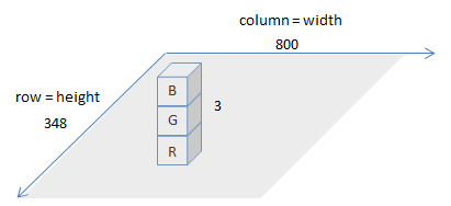
As the name of cv2.COLOR_BGR2GRAY suggests, the color information of the image loaded by cv2.imread is loaded in the order of BGR (blue-green-red). The variable that read the image is a matrix (of numpy), but if you check its size, it is as follows.

img = cv2.imread(IMAGE_PATH)
img.shape
>>> (348, 800, 3)

This means that the loaded image is represented by a 348x800x3 matrix. The image looks like the figure below.

In addition, matplotlib, which is often used to display images, expects images to come in in RGB. Therefore, if you put the image read by OpenCV into matplotlib as it is, it will be as follows (the original image is on the left, the one read by OpenCV is displayed by matplotlib as it is).

Image Source

Therefore, when displaying with matplotlib, it is necessary to change the order of colors as follows.

def to_matplotlib_format(img):
    return cv2.cvtColor(img, cv2.COLOR_BGR2RGB)

Threshold processing

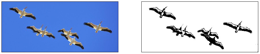
Threshold processing is image processing based on whether or not a certain threshold is exceeded. For example, it is a process such as setting all areas where the brightness does not reach a certain value to 0. This makes it possible to drop the background and emphasize the outline, and process it as shown in the figure below (the left side is the original image, the right side is the one with threshold processing).

Threshold processing in OpenCV is executed by cv2.threshold can. The main parameters here are the threshold thresh, the upper limit of the value maxval, and the threshold processing type type.

The table below summarizes the types of type for threshold treatment and how the threshold (thresh) / upper limit (maxValue) is used at that time.

Threshold Type	over thresh :arrow_up_small:	under thresh :arrow_down_small:
`THRESH_BINARY`	maxValue	0
`THRESH_BINARY_INV`	0	maxValue
`THRESH_TRUNC`	threshold	(as is)
`THRESH_TOZERO`	(as is)	0
`THRESH_TOZERO_INV`	0	(as is)

(as is) means that the value of the original image is used as is. If you want to know more about threshold processing, the following materials will be helpful.

OpenCV Threshold ( Python , C++ )

In the bird image used this time, in addition to removing the blue background, the boundary (bright) of the bird's wings is made clear.

Drop the background-> THRESH_BINARY
Areas larger than the threshold (= bright = light = background): maxValue (255 = white = erase)
Below threshold: 0 (black = emphasized)
Clarification of boundaries-> THRESH_BINARY_INV
Areas larger than the threshold (= bright = bird bone = boundary): 0 (black = emphasized)
Below threshold: maxValue (255 = white = erase)

And finally, these two processing results are merged.

def binary_threshold(path):
    img = cv2.imread(path)
    grayed = cv2.cvtColor(img, cv2.COLOR_BGR2GRAY)
    under_thresh = 105
    upper_thresh = 145
    maxValue = 255
    th, drop_back = cv2.threshold(grayed, under_thresh, maxValue, cv2.THRESH_BINARY)
    th, clarify_born = cv2.threshold(grayed, upper_thresh, maxValue, cv2.THRESH_BINARY_INV)
    merged = np.minimum(drop_back, clarify_born)
    return merged

If you are not sure what the value of thresh should be, you can check the brightness with a paint tool. On Windows, you can check it with the standard paint tool dropper.

If you use ʻadaptiveThreshold`, it will determine an appropriate threshold while looking at the surrounding pixels, so you may want to try it once. Please refer to the following document for details.

Image Thresholding

Threshold processing by color

Specific colors using cv2.inRange It is also possible to extract the part of. In the following, the blue part of the background is detected and masked.

def mask_blue(path):
    img = cv2.imread(path)
    hsv = cv2.cvtColor(img, cv2.COLOR_BGR2HSV)

    blue_min = np.array([100, 170, 200], np.uint8)
    blue_max = np.array([120, 180, 255], np.uint8)
    
    blue_region = cv2.inRange(hsv, blue_min, blue_max)
    white = np.full(img.shape, 255, dtype=img.dtype)
    background = cv2.bitwise_and(white, white, mask=blue_region)  # detected blue area becomes white
    
    inv_mask = cv2.bitwise_not(blue_region)  # make mask for not-blue area
    extracted = cv2.bitwise_and(img, img, mask=inv_mask)
    
    masked = cv2.add(extracted, background)
    
    return masked

The blue_region obtained by cv2.inRange is the specified color region. Note that blue_region is represented in grayscale, with higher values (255 = closer to white) where it is found. In addition, when using cv2.inRange, it is necessary to change the image to HSV representation, and it is also necessary to specify the color range accordingly. What is HSV expression? It is easy to understand by looking at the figure below.

HSL and HSV

However, the value of HSV specified by OpenCV is a little quirky, so it is quite difficult to estimate the value from the paint tool as described above.

	General range of values	OpenCV
H	0 - 360	0 - 180
S	0 - 100	0 - 255
V	0 - 100	0 - 255

Therefore, it is faster to actually look at the values in the matrix if the specification does not seem to work very well. You can cut out the matrix value (color value) of the specified area with the feeling of ʻimg [10:20, 10:20] `, so if you check it, you can specify it pinpointly (in fact, this time the paint value is It didn't help at all, so I specified it this way).

After that, the image is created by adding background, which makes the area of blue_region all white, and ʻextracted, which extracts the area other than blue_region. bitwise_and / bitwise_not` is a useful function for doing this kind of masking.

The above is the explanation of threshold processing.

Smoothing

If the outline of the image is not clear or the background is dark, the outline may not be removed or the background may remain even if threshold processing is applied. In the example below, the gravel at your feet remains fine and the outline is jagged.

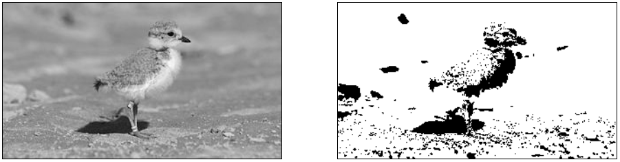Piping plover chick with band at two weeks

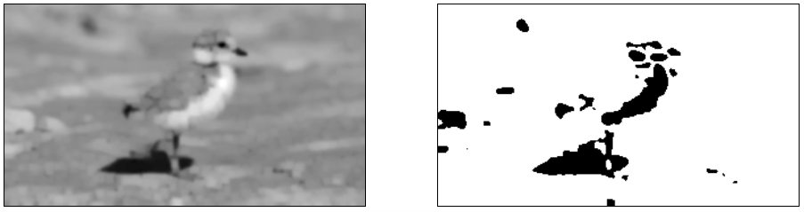
In such cases, it is a good idea to use a filter for smoothing. To put it simply, filtering is a process that blurs an image, but by blurring an image, it is possible to detect only "points that are clearly visible even if they are blurred" and ignore points that disappear if they are blurred. I can do it. The following is an example of applying a Gaussian filter using Gaussian Blur (left figure) and then performing threshold processing (right figure).

def blur(img):
    filtered = cv2.GaussianBlur(img, (11, 11), 0)
    return filtered

The fine details of the image have been lost, but you can see that the characteristic parts remain together and the noise that was often in the background has disappeared. Please refer to the following OpenCV official documentation for filters other than Gaussian Blur.

Smoothing Images

Another technique used to smooth images is morphology. This is a method of removing noise and emphasizing contours by using image expansion / contraction processing. The following is an image of a typical method in morphology.

Morphology

Dialation: Has the effect of expanding the border area
Erosion: Has the effect of eroding the border area
Opening: Similar to Erosion, eroding boundaries but slower than Erosion.
Closing: Similar to Dialation, expanding boundaries and shrinking the background, but slower than Dialation

The theoretical details are omitted here, but you can think of it as a type of filter. OpenCV has cv2.dilate, cv2.erode which can perform the above morphology processing, and convenient cv2.morphologyEx which can apply Opening / Closing continuously. This time, I will use cv2.morphologyEx to perform smoothing.

def morph(img):
    kernel = np.ones((3, 3),np.uint8)
    opened = cv2.morphologyEx(img, cv2.MORPH_OPEN, kernel, iterations=2)
    return opened

This time, probably because the background color is dark, it became difficult to thicken the area with CLOSE, so I tried processing in the direction of making the distance between the areas as large as possible by OPEN. However, since noise still remains, it is processed in combination with a filter.

def morph_and_blur(img):
    kernel = np.ones((3, 3),np.uint8)
    m = cv2.GaussianBlur(img, (3, 3), 0)
    m = cv2.morphologyEx(m, cv2.MORPH_OPEN, kernel, iterations=2)
    m = cv2.GaussianBlur(m, (5, 5), 0)
    return m

It's more like information remains than simply filtering. Also, you can see that the areas that were previously connected are now firmly independent by applying Opening. The following is detailed about morphology processing, so please refer to it.

In fact, when the background is dark, it is quite difficult to clarify the area from there if it is grayscale. Therefore, if the background has a color that you can recognize, it is better to mask it with a color and then process it.

The above is the explanation of preprocessing. From here, I would like to finally detect the object from the image after preprocessing.

Object detection

Contour detection

Up to this point, I think that the object to be recognized has been clarified by preprocessing, so we will use it to detect the contour.

In OpenCV, you can easily detect contours by using cv2.findContours.

def detect_contour(path, min_size):
    contoured = cv2.imread(path)
    forcrop = cv2.imread(path)

    # make binary image
    birds = binary_threshold_for_birds(path)
    birds = cv2.bitwise_not(birds)
    
    # detect contour
    im2, contours, hierarchy = cv2.findContours(birds, cv2.RETR_EXTERNAL, cv2.CHAIN_APPROX_SIMPLE)
    
    crops = []
    # draw contour
    for c in contours:
        if cv2.contourArea(c) < min_size:
            continue
        
        # rectangle area
        x, y, w, h = cv2.boundingRect(c)
        x, y, w, h = padding_position(x, y, w, h, 5)
        
        # crop the image
        cropped = forcrop[y:(y + h), x:(x + w)]
        cropped = resize_image(cropped, (210, 210))
        crops.append(cropped)
        
        # draw contour
        cv2.drawContours(contoured, c, -1, (0, 0, 255), 3)  # contour
        cv2.rectangle(contoured, (x, y), (x + w, y + h), (0, 255, 0), 3)  #rectangle contour
                
    return contoured, crops


def padding_position(x, y, w, h, p):
    return x - p, y - p, w + p * 2, h + p * 2

binary_threshold_for_birds is a function for threshold processing of the bird image used this time (= preprocessing). Since the image output with this is the white background image introduced earlier, this is inverted and used for area detection. It is difficult to understand, but in the case of black and white, "white" has a higher value (255), so when performing contour detection, it is necessary to give an image whose contour is drawn in white as input.

Please note that the outline will not be detected unless the image is fairly clear in black and white.

All you have to do now is run cv2.findContours. The contours detected by this can be easily drawn on the image with cv2.drawContours. You can also use cv2.boundingRect to get the coordinates of a rectangle that fits the contour. However, this is a close battle, so this time I'm using padding_position to give some room to the surroundings. For cv2.findContours, please refer to the official document as well.

Contours : Getting Started

In addition, when the user is not automatic, it is possible to detect the object in the enclosed area by using a technique called graph cut. I won't go into details, but I think it's useful when creating tools for annotation, so if you are interested, please refer to the following.

Interactive Foreground Extraction using GrabCut Algorithm

Approximation of contour

OpenCV provides several functions that approximate the detected contour. For example, ʻapproxPolyDP` linearly approximates the detected contour, and if the contour is straight, it is recommended to use this to cut out. Below is the contour detected by the red dotted line, and the green line is a straight line approximation.

Image source

def various_contours(path):
    color = cv2.imread(path)
    grayed = cv2.cvtColor(color, cv2.COLOR_BGR2GRAY)
    _, binary = cv2.threshold(grayed, 218, 255, cv2.THRESH_BINARY)
    inv = cv2.bitwise_not(binary)    
    _, contours, _ = cv2.findContours(inv, cv2.RETR_EXTERNAL, cv2.CHAIN_APPROX_SIMPLE)
    
    for c in contours:
        if cv2.contourArea(c) < 90:
            continue
        
        epsilon = 0.01 * cv2.arcLength(c, True)
        approx = cv2.approxPolyDP(c, epsilon, True)
        cv2.drawContours(color, c, -1, (0, 0, 255), 3)
        cv2.drawContours(color, [approx], -1, (0, 255, 0), 3)
        
    plt.imshow(cv2.cvtColor(color, cv2.COLOR_BGR2RGB))
    
various_contours(IMG_FOR_CONTOUR)

cv2.arcLength is the length of the contour, which is used to calculate the minimum straight line length ʻepsilon`. Now you can adjust how fine the straight line is. For other functions, please refer to the tutorial below for how to use and explain them.

Contour Features

Cutting out the detection area

Now that we know the area, in order to apply it to a machine learning model, we need to cut it out to the size that the model expects. To do this, I created a function called resize_image this time.

def resize_image(img, size):
    # size is enough to img
    img_size = img.shape[:2]
    if img_size[0] > size[1] or img_size[1] > size[0]:
        raise Exception("img is larger than size")
    
    # centering
    row = (size[1] - img_size[0]) // 2
    col = (size[0] - img_size[1]) // 2
    resized = np.zeros(list(size) + [img.shape[2]], dtype=np.uint8)
    resized[row:(row + img.shape[0]), col:(col + img.shape[1])] = img
        
    # filling
    mask = np.full(size, 255, dtype=np.uint8)
    mask[row:(row + img.shape[0]), col:(col + img.shape[1])] = 0
    filled = cv2.inpaint(resized, mask, 3, cv2.INPAINT_TELEA)    
    
    return filled

This function is formed by the following steps.

resize: Prepare a canvas (resized) of a predetermined size (size the image of the training data or make it a little larger so that it will be cut out later)
centering: Set the cut out image in the center of the prepared canvas
filling: Fills the peripheral area of the set image using the information of the original image.

OpenCV also has a resize function, but if you use it, the cropped image will be forcibly adjusted to the specified size, and the image will be distorted. Therefore, this time, we take a method of preparing a canvas of a size that fits the cut out image, placing the cut out image in the center, and filling the surroundings. Cv2.inpaint used to fill in the blanks is originally a function to restore defects in the image. However, this time I am using it to fill the surroundings.

The image actually cut out is as follows. I think that it is almost exactly complemented, but the color of the beak on the second piece has grown a little. In these cases, you need to adjust the padding so that it is filled with just the background color.

Image alignment

The position on the image where the object is moved is an important point in recognition. CNN, which is used recently, will do it well even if it is slightly misaligned due to convolution, but if you correct it, the accuracy will be greatly improved. Therefore, here we will explain the position correction of the image after cropping.

The figure below is an example of aligning the images. The first row is the base image, and the second and subsequent rows are corrected to align with the first row image (the left side is before correction, the right side is after correction).

Image Source: image 1, [image 2](http://www.publicdomainpictures.net/view- image.php? image = 51893 & picture = & jazyk = JP), image 3

After applying the correction, I think that the positions of the birds are almost the same. This is corrected using findTransformECC referring to the following site.

Image Alignment (ECC) in OpenCV ( C++ / Python )

def align(base_img, target_img, warp_mode=cv2.MOTION_TRANSLATION, number_of_iterations=5000, termination_eps=1e-10):
    base_gray = cv2.cvtColor(base_img, cv2.COLOR_BGR2GRAY)
    target_gray = cv2.cvtColor(target_img, cv2.COLOR_BGR2GRAY)
    
    # prepare transformation matrix
    if warp_mode == cv2.MOTION_HOMOGRAPHY:
        warp_matrix = np.eye(3, 3, dtype=np.float32)
    else :
        warp_matrix = np.eye(2, 3, dtype=np.float32)
    
    criteria = (cv2.TERM_CRITERIA_EPS | cv2.TERM_CRITERIA_COUNT, number_of_iterations,  termination_eps)
    sz = base_img.shape
    
    # estimate transformation
    try:
        (cc, warp_matrix) = cv2.findTransformECC(base_gray, target_gray, warp_matrix, warp_mode, criteria)

        # execute transform
        if warp_mode == cv2.MOTION_HOMOGRAPHY :
            # Use warpPerspective for Homography 
            aligned = cv2.warpPerspective(target_img, warp_matrix, (sz[1], sz[0]), flags=cv2.INTER_LINEAR + cv2.WARP_INVERSE_MAP)
        else :
            # Use warpAffine for Translation, Euclidean and Affine
            aligned = cv2.warpAffine(target_img, warp_matrix, (sz[1],sz[0]), flags=cv2.INTER_LINEAR + cv2.WARP_INVERSE_MAP)
    
        return aligned
    except Exception as ex:
        print("can not align the image")
        return target_img

findTransformECC is simply a function that looks for similarities between two images and puts the estimation result of what kind of movement was done in warp_matrix. Originally, it is for analyzing what kind of movement occurred on continuous frames such as movies, so the positions may not be aligned unless the images are quite the same. The above also seem to be casually aligned, but it was difficult to choose a photo that could be correlated (the exception is that if there is no correlation, it will not converge). .. ..

If there are feature points (eyes, nose, mouth, etc.) that are common to all images such as the face, conversion can be applied based on the position of each feature point. ʻEstimateRigidTransform` can be used for this.

def face_align(base, base_position, target, target_position):
    sz = base.shape
    fsize = min(len(base_position), len(target_position))  # adjust feature size
    tform = cv2.estimateRigidTransform(target_position[:fsize], base_position[:fsize], False)
    aligned = cv2.warpAffine(target, tform, (sz[1], sz[0]))
    return aligned

Since there are cases where the eyes cannot be detected depending on the photo, the conversion is performed according to the smaller detected feature amount in the above (however, please note that in this case, the order in which the feature amount is inserted must be aligned. ).

Image source

After the conversion, you can see that the positions of the faces are aligned. There is also a detailed introduction to face alignment below, so please refer to it.

Average Face : OpenCV ( C++ / Python ) Tutorial

Object recognition

In the above, contour detection was performed by itself, but OpenCV has a trained model for objects that often detect objects such as faces and bodies, and object recognition can be performed by using this. This trained model file is called Cascade Classifier, and you can also create your own. There are some that are open to the public, so if you are interested, please refer to them as they are summarized below.

Cascade Classifier is in (virtual environment folder) \ Library \ etc \ haarcascades when installed with pip (for Windows / miniconda. I think it depends on the environment). You may want to experiment to see if there is something that seems to suit your purpose. This time, I would like to follow the official tutorial below to detect faces.

Face Detection using Haar Cascades

The result of the actual detection is as follows. The detection of the right eye has failed probably because it is hidden by the hair. .. ..

Image source

The code is almost as per the tutorial. Please note that the location of the Cascade File depends on the environment as described above (if the path is not successful, you will get an error such as ʻerror: (-215)! Empty () in function`).

def face_detection(path):
    face_cascade = cv2.CascadeClassifier(CASCADE_DIR + "/haarcascade_frontalface_default.xml")
    eye_cascade = cv2.CascadeClassifier(CASCADE_DIR + "/haarcascade_eye.xml")
    
    img = cv2.imread(path)
    grayed = cv2.cvtColor(img, cv2.COLOR_BGR2GRAY)
    
    faces = face_cascade.detectMultiScale(grayed, 1.3, 5)
    for (x, y, w, h) in faces:
        img = cv2.rectangle(img, (x, y), (x + w, y + h), (255, 0, 0), 2)
        roi_gray = grayed[y:y+h, x:x+w]
        roi_color = img[y:y+h, x:x+w]
        eyes = eye_cascade.detectMultiScale(roi_gray)
        for (ex, ey, ew, eh) in eyes:
            cv2.rectangle(roi_color, (ex,ey), (ex + ew, ey + eh), (0, 255, 0), 2)

    plt.imshow(cv2.cvtColor(img, cv2.COLOR_BGR2RGB))

face_detection(IMG_FACE)

The basic flow is to read the file with cv2.CascadeClassifier, create Classifier, and detect with detectMultiScale. This time, only grayscale is used, but I think that more reliable detection can be achieved by performing the above-mentioned threshold processing. For cutting out the detected part, refer to "Cut out the detection area" in the previous section.

If the face is tilted, it will not be detected properly. There are two ways to do this: the eye / mouth is detected first to determine the tilt, or the image is simply rotated gradually to attempt detection. The trade-off is that the former is less computationally complicated but cumbersome, and the latter is easier but more computationally expensive. The following describes in detail the method of detecting while rotating the image, so please refer to it.

Preparing for learning

Up to this point, you have been able to cut out an image of the target object from the image. All you have to do now is put the collected images into a machine learning model. However, various preprocessing is required when inputting images to the learning model. This point is summarized below.

[Implementing Convolutional Neural Network / Preprocessing data](http://qiita.com/icoxfog417/items/5aa1b3f87bb294f84bac#%E3%83%87%E3%83%BC%E3%82%BF%E3%81] % AE% E5% 89% 8D% E5% 87% A6% E7% 90% 86)

To extract the points, the following processing is required.

Matrix transformation: Convert to the matrix format (usually K (depth = color) x H (height) x W (width)) that the training model expects.
Depth adjustment: Convert to the color channel that the training model expects (grayscale or RGB)
Normalize image data: Create an average image by averaging all images and normalize the image.
Scaling: Converts the price range from 0 to 255 to 0 to 1.

That is all for the explanation. Please use OpenCV well and let them learn various things.

[PYTHON] An introduction to OpenCV for machine learning

Preprocessing

Grayscale

Threshold processing

Threshold processing by color

Smoothing

Object detection

Contour detection

Approximation of contour

Cutting out the detection area

Image alignment

Object recognition

Preparing for learning

References