[PYTHON] Introduction to Statistical Modeling for Data Analysis Expanding the range of applications of GLM
We deal with offset term works of logistic regression and Poisson regression, and GLM using normal distribution and gamma distribution.
GLM to which various types of data can be applied
Various types of data can be represented by GLM by combining probability distributions, link functions, and linear predictors.
Part of the probability distribution that can be used to build GLM in Python
Random number generation is specified by scipy.stats.X, and glm () family is specified by statsmodels.api.families.X.
| Probability distribution | Random number generation | glm()Family designation | Frequently used link functions | |
|---|---|---|---|---|
| (Discrete) | Binomial distribution | binom.rvs() | Binomial() | logit |
| Poisson distribution | poisson.rvs() | Poisson() | log | |
| Negative binomial distribution | nbinom.rvs() | NegativeGaussian() | log | |
| (Continuous) | Gamma distribution | gamma.rvs() | Ganma() | log? |
| normal distribution | norm.rvs() | Gaussian() | identity |
GLM with binomial distribution
The binomial distribution is used when ** count data with an upper limit ** (response variable is $ y \ in \ {0, 1, 2, \ dots, N \} $).
When the same treatment was applied to the experimental subjects of N individuals, the reaction was positive in $ y $ individuals and negative in $ N-y $ individuals.
This example is
"For each $ i $ of a fictitious plant, $ y_i $ of live and germinated seeds and $ N_i-y_i $ of dead seeds of $ N_i $ observed seeds."
Suppose that a total of 100 plants were investigated using the observation data.
- The number of observed seeds $ N_i $ is 8 for any individual.
About response variables
The possible value of the number of surviving seeds, which is the response variable, is $ y_i \ in \ {0, 1, 2, 3, \ dots, 8 \} $. If all are alive, $ y_i = 8 $, and if all the meanings are dead, $ y_i = 0 $.
Let $ q_i $ be the "probability that one seed obtained from a certain individual $ i $ is alive".
About explanatory variables
The survival probability $ q_i $ fluctuates depending on the body size $ x_i
>>> import pandas
>>> import matplotlib.pyplot as plt
>>> d = pandas.read_csv("data4a.csv")
>>> d.describe()
         N           y           x
count  100  100.000000  100.000000
mean     8    5.080000    9.967200
std      0    2.743882    1.088954
min      8    0.000000    7.660000
25%      8    3.000000    9.337500
50%      8    6.000000    9.965000
75%      8    8.000000   10.770000
max      8    8.000000   12.440000
>>> plt.plot(d.x[d.f == 'C'], d.y[d.f == 'C'], 'bo')
>>> plt.plot(d.x[d.f == 'T'], d.y[d.f == 'T'], 'ro')
>>> plt.show()

As you can see from the figure
--It seems that the number of surviving seeds $ y_i $ increases as the body size $ x_i $ increases. --It seems that fertilizer ($ f_i = T $) will increase the number of surviving seeds $ y_i $.
Binomial distribution
p(y|N, q) = \left( \begin{array}{c}
      N \\
      y
    \end{array}
    \right) q^y (1-q)^{N-y}
>>> import math
>>> p = lambda y, N, q: (math.factorial(N) / (math.factorial(y) * math.factorial(N-y))) * (q ** y) * ((1-q) ** (N-y))
>>> p1 = [p(i, 8, 0.1) for i in y]
>>> p2 = [p(i, 8, 0.3) for i in y]
>>> p3 = [p(i, 8, 0.8) for i in y]
>>> plt.plot(y, p1, 'b-o')
>>> plt.plot(y, p2, 'r-o')
>>> plt.plot(y, p3, 'g-o')
>>> plt.show()

Logistic regression and logit link functions
In logistic regression
--Probability distribution: ** Binomial distribution ** --Link function: ** logit link function **
Is used.
About ** logistic function **
q_i = logistic(z_i) = \frac{1}{1+\exp(-z_i)}
The variable $ z_i $ is the linear predictor $ z_i = \ beta_1 + \ beta_2 x_1 + \ dots $.
>>> logistic = lambda z: 1 / (1 + numpy.exp(-z))
>>> z = numpy.arange(-6, 6, 0.1)
>>> plt.plot(z, logistic(z))
>>> plt.show()

Assuming that the survival probability $ q_i $ is a logistic function of $ z_i $, any value of the linear predictor $ z_i $ will be $ 0 \ leq q_i \ leq 1 $.
Assuming that the survival probability $ q_i $ depends only on the body size $ x_i $, we have the linear predictor $ z_i = \ beta_1 + \ beta_2 x_i $.
$ Q_i $ and $ x_i $ depend on $ \ beta_1 $ and $ \ beta_2 $
>>> plt.subplot(121)
>>> logistic = lambda x: 1 / (1 + numpy.exp(-(0 + 2 * x)))
>>> plt.plot(z, logistic(z), 'b-', label='beta1=0')
>>> logistic = lambda x: 1 / (1 + numpy.exp(-(2 + 2 * x)))
>>> plt.plot(z, logistic(z), 'r-', label='beta1=2')
>>> logistic = lambda x: 1 / (1 + numpy.exp(-(-3 + 2 * x)))
>>> plt.plot(z, logistic(z), 'g-', label='beta1=-3')
>>> plt.legend(loc='middle right')
>>> plt.subplot(122)
>>> logistic = lambda x: 1 / (1 + numpy.exp(-(2 * x)))
>>> plt.plot(z, logistic(z), 'b-', label='beta2=2')
>>> logistic = lambda x: 1 / (1 + numpy.exp(-(4 * x)))
>>> plt.plot(z, logistic(z), 'r-', label='beta2=4')
>>> logistic = lambda x: 1 / (1 + numpy.exp(-(-1 * x)))
>>> plt.plot(z, logistic(z), 'g-', label='beta2=-1')
>>> plt.legend(loc='middle right')
>>> plt.show()

Logit function
Transform the logistic function.
\begin{eqnarray}
q_i &=& \frac{1}{1+\exp(-z_i)} \\
q_i + q_i \exp(-z_i) &=& 1 \\
1 - q_i &=& q_i \exp (-z_i)\\
\frac{1 - q_i}{q_i} &=& \exp (-z_i) \\
\log \frac{1 - q_i}{q_i} &=& -z_i \\
\log \frac{q_i}{1 - q_i} &=& z_i
\end{eqnarray}
The left side is called the ** logit function **.
logit(q_i) = \log \frac{q_i}{1 - q_i}
- The logit function is the inverse of the logistic function.
Parameter estimation
Maximize the (logarithmic) likelihood under the survival probability $ q_i $.
\begin{eqnarray}
L(q) &=& \prod_i p(y_i | N_i, q_i) \\
&=& \prod_i \left( \begin{array}{c}
      N_i \\
      y_i
    \end{array}
    \right)q_i^{y_i}(1-q_i)^{N_i-y_i} \\
L(\{\beta_1, \beta_2, \beta_3\}) &=& \prod_i \left( \begin{array}{c}
      N_i \\
      y_i
    \end{array}
    \right)q_i^{y_i}(1-q_i)^{N_i-y_i} (\because logit(q_i) = z_i = \beta_1 + \beta_2 x_i + \beta_3 d_i) \\
logL(\{\beta_1, \beta_2, \beta_3\}) &=& \sum_i \log \left\{\left( \begin{array}{c}
      N_i \\
      y_i
    \end{array}
    \right)q_i^{y_i}(1-q_i)^{N_i-y_i} \right\} \\

logL(\{\beta_1, \beta_2, \beta_3\}) &=& \sum_i \left\{ \log \left( \begin{array}{c}
      N_i \\
      y_i
    \end{array}
    \right) + \log q_i^{y_i} + \log (1-q_i)^{N_i-y_i} \right\} \\

logL(\{\beta_1, \beta_2, \beta_3\}) &=& \sum_i \left\{ \log \left( \begin{array}{c}
      N_i \\
      y_i
    \end{array}
    \right) + (y_i)\log q_i + (N_i-y_i)\log (1-q_i) \right\} \\
\end{eqnarray}
>>> import statsmodels.formula.api as smf
>>> import statsmodels.api as sm
>>> import pandas
>>> d = pandas.read_csv("data4a.csv")
# glm(cbind(y, N-y) ~ x + f, data=d, family=binomial)
>>> model = smf.glm('y + I(N-y) ~ x + f', data=d, family=sm.families.Binomial())
>>> fit = model.fit()
>>> fit.summary()
                 Generalized Linear Model Regression Results
==============================================================================
Dep. Variable:      ['y', 'I(N - y)']   No. Observations:                  100
Model:                            GLM   Df Residuals:                       97
Model Family:                Binomial   Df Model:                            2
Link Function:                  logit   Scale:                             1.0
Method:                          IRLS   Log-Likelihood:                -133.11
Date:                Sat, 06 Jun 2015   Deviance:                       123.03
Time:                        12:06:47   Pearson chi2:                     109.
No. Iterations:                     8
==============================================================================
                 coef    std err          z      P>|z|      [95.0% Conf. Int.]
------------------------------------------------------------------------------
Intercept    -19.5361      1.414    -13.818      0.000       -22.307   -16.765
f[T.T]         2.0215      0.231      8.740      0.000         1.568     2.475
x              1.9524      0.139     14.059      0.000         1.680     2.225
==============================================================================

About odds
The ratio of (probability of survival) / (probability of non-survival) is called ** odds **.
\begin{eqnarray}
\frac{q_i}{1-q_i} &=& \exp(Linear predictor) \\
&=& \exp(\beta_1 + \beta_2 x_i + \beta_3 f_i) \\
&=& \exp(\beta_1)\exp(\beta_2 x_i)\exp(\beta_3 f_i)
\end{eqnarray}
Focusing on the $ \ {\ beta_2, \ beta_3 \} $ estimated this time
\frac{q_i}{1-q_i} \propto \exp(1.95x_i)\exp(2.02f_i)
And each explanatory variable have a proportional relationship.
The effect of body size $ x_i $ is
\begin{eqnarray}
\frac{q_i}{1-q_i} &\propto& \exp(1.95(x_i + 1))\exp(2.02f_i) \\
&\propto& \exp(1.95x_i)\exp(1.95)\exp(2.02f_i)
\end{eqnarray}
It can be seen from that $ \ exp (1.95) \ approach 7.03 $ times. Similarly, it can be seen that the fertilizer application effect is $ exp (2.02) \ approx 7.54 $ times.
About odds ratio
The effect of factor $ X $ ($ \ beta_x = 1.95 $) is shown.
\begin{eqnarray}
\frac{X odds}{非X odds} &=& \frac{\exp(X\bullet Non-X intersection)\times \exp(1.95 \times 1)}{\exp(X\bullet Non-X intersection)\times \exp(1.95 \times 0)} \\
&=& exp(1.95) \approx 7.03
\end{eqnarray}
Model selection
Model selection by AIC Selection of nested models for logistic regression
--Constant model (intercept only) --x model (body size only) --f model (fertilization effect only) --x + f model (body size + fertilizer application effect)
It seems that R has the stepAIC () function of the MASS package.
For the time being, if the same as the last time, the x + f model has the lowest AIC and is a good model.
Interaction term
Consider the effect of multiplying the body size and the fertilizer application effect. In other words
logit(q_i) = \beta_1 + \beta_2 x_i + \beta_3 f_i + \beta_4 x_i f_i
think of.
# glm(cbind(y, N-y) ~ x * f, data=d, family=binomial)
>>> model = smf.glm('y + I(N-y) ~ x * f', data=d, family=sm.families.Binomial())
>>> model.fit().summary()
                 Generalized Linear Model Regression Results
==============================================================================
Dep. Variable:      ['y', 'I(N - y)']   No. Observations:                  100
Model:                            GLM   Df Residuals:                       96
Model Family:                Binomial   Df Model:                            3
Link Function:                  logit   Scale:                             1.0
Method:                          IRLS   Log-Likelihood:                -132.81
Date:soil, 06  6 2015   Deviance:                       122.43
Time:                        13:44:31   Pearson chi2:                     13.6
No. Iterations:                     8
==============================================================================
                 coef    std err          z      P>|z|      [95.0% Conf. Int.]
------------------------------------------------------------------------------
Intercept    -18.5233      5.335     -3.472      0.001       -28.979    -8.067
f[T.T]        -0.0638      7.647     -0.008      0.993       -15.052    14.924
x              1.8525      0.525      3.529      0.000         0.824     2.881
x:f[T.T]       0.2163      0.792      0.273      0.785        -1.336     1.769
==============================================================================
This time, the AIC went up, so there was no interaction.
Stop statistical modeling of division values
One of the merits of logistic regression is that it is not necessary to create a division value of $ (observation data) / (observation data) $. The division place tends to be created when you want to know "what the survival probability of seeds depends on" in this example.
As a disadvantage
-** Information is lost : Baseball batting average as an example. 300 hits in 1000 at bats and 30 hits in 100 at bats are both 30% hitters, but can we say that they are equally certain? - What is the distribution of the converted values? **: What probability distribution does the division value created by the quantities with errors follow?
Offset term work that does not require a division value
Use fictitious data such as
--100 survey sites have been set up around the forest ($ i \ in \ {1, 2, \ dots, 100 \} $) --The area $ A_i $ is different for each survey site $ i $ --Measuring the "brightness" $ x_i $ of the survey site $ i $ --Recorded the number of plant populations $ y_i $ at the survey site $ i $ -(Purpose of analysis) I would like to know how the "population density" of individual plants at the survey site $ i $ is affected by "brightness" $ x_i $.
The population density at the survey site $ i $, which has an area of $ A_i $, is
\frac{Average population\lambda_i}{A_i} =Population density
Is. Population density is a positive quantity, so combine the exponential function with the brightness $ x_i $ dependence,
\begin{eqnarray}
\lambda_i &=& A_i \times Population density\\
&=& A_i \exp(\beta_1 + \beta_2 x_i) \\
&=& \exp(\beta_1 + \beta_2 x_i + \log A_i)
\end{eqnarray}
Therefore, it becomes a GLM of the logarithmic link function Poisson distribution with $ z_i = \ beta_1 + \ beta_2 x_i + \ log A_i $ as the linear predictor.
>>> d = pandas.read_csv("data4b.csv")
>>> model = smf.glm('y ~ x', offset=numpy.log(d.A), data=d, family=sm.families.Poisson())
>>> model.fit().summary()
                 Generalized Linear Model Regression Results
==============================================================================
Dep. Variable:                      y   No. Observations:                  100
Model:                            GLM   Df Residuals:                       98
Model Family:                 Poisson   Df Model:                            1
Link Function:                    log   Scale:                             1.0
Method:                          IRLS   Log-Likelihood:                -323.17
Date:                Sat, 06 Jun 2015   Deviance:                       81.608
Time:                        14:45:24   Pearson chi2:                     81.5
No. Iterations:                     7
==============================================================================
                 coef    std err          z      P>|z|      [95.0% Conf. Int.]
------------------------------------------------------------------------------
Intercept      0.9731      0.045     21.600      0.000         0.885     1.061
x              1.0383      0.078     13.364      0.000         0.886     1.191
==============================================================================
Normal distribution and its likelihood
Probability distribution for handling continuous value data in a statistical model. It is also called ** Gaussian distribution **.
The parameters are
--Mean value $ \ mu $: Can be changed freely within the range of $ \ pm \ infinity $. --Standard deviation $ \ sigma $: Data variation can be specified.
p(y| \mu, \sigma) = \frac{1}{\sqrt{2\pi\sigma^2}}\exp \left\{ -\frac{(y-\mu)^2}{2\sigma^2} \right\}
# y <- seq(-5, 5, 0.1)
# plot(y, dnorm(y, mean=0, sd=1), type="l")
plt.subplot(131)
plt.plot(y, sct.norm.pdf(y, loc=0, scale=1))
plt.title('$\mu=0, \sigma=1$')
plt.subplot(132)
plt.plot(y, sct.norm.pdf(y, loc=0, scale=3))
plt.title('$\mu=0, \sigma=3$')
plt.subplot(133)
plt.plot(y, sct.norm.pdf(y, loc=2, scale=1))
plt.title('$\mu=2, \sigma=1$')
plt.show()
In R, $ \ mu $ is
meanand $ \ sigma $ issd. In python, $ \ mu $ islocand $ \ sigma $ isscale.

Each parameter is adjusted. The vertical axis shows ** probability density **. The area painted in red is represented by the magnitude of the probability of becoming $ 1.2 \ leq y \ leq 1.8 $.
Let $ p (y | \ mu, \ sigma) $ be the probability density function of the normal distribution.
$p(1.2 \leq y \leq 1.8| \mu, \sigma) = \int_{1.2}^{1.8}p(y| \mu, \sigma)dy
#Cumulative distribution
# pnorm(1.8, 0, 1) - pnorm(1.2, 0, 1)
>>> sct.norm.cdf(1.8, 0, 1) - sct.norm.cdf(1.2, 0, 1)
0.079139351108782452
Since the probability is an area, it is approximated as a rectangle. In this case, if the height is $ p (y = 1.5 | 0, 1) $ and the width is $ \ Delta y = 1.8-1.2 = 0.6 $,
#Probability density
# dnorm(1.5, 0, 1) * 0.6
>>> sct.norm.pdf(1.5, 0, 1) * 0.6
0.077710557399535043
It can be seen that the approximation is made.
Maximum likelihood estimation
Based on $ probability = probability density function \ times \ Delta y $.
Let the height data of a human group of $ N $ be $ {\ bf Y} = \ {y_i \} $. The probability that a $ y_i $ is $ y_i-0.5 \ Delta y \ leq y_i \ leq y_i + 0.5 \ Delta y $ is the probability density function $ p (y_i | 0, 1) $ and the interval width $ \ Delta y $. Because it can be approximated as a seat of The (logarithmic) likelihood function of a statistical model using a normal distribution is.
\begin{eqnarray}
L(\mu, \sigma) &=& \prod_i p(y_i|\mu, \sigma)\times \Delta y \\
&=& \prod_i \frac{1}{\sqrt{2\pi\sigma^2}}\exp \left\{ -\frac{(y-\mu)^2}{2\sigma^2}\right\}  \Delta y \\
log L(\mu, \sigma) &=& \sum_i \left\{-\log \sqrt{2\pi\sigma^2} + \log \Delta y - \frac{(y-\mu)^2}{2\sigma^2}    \right\} \\
&=& -0.5N\log(2\pi\sigma^2) + N\log \Delta y - \frac{1}{2\sigma^2}\sum_i (y-\mu)^2
\end{eqnarray}
It becomes. Note that $ \ Delta y $ is a constant and does not affect the parameter $ \ {\ mu, \ sigma \} $. Ignore the above equation. Therefore,
log L(\mu, \sigma) = -0.5N\log(2\pi\sigma^2) - \frac{1}{2\sigma^2}\sum_i (y-\mu)^2
It becomes.
Gamma distribution GLM
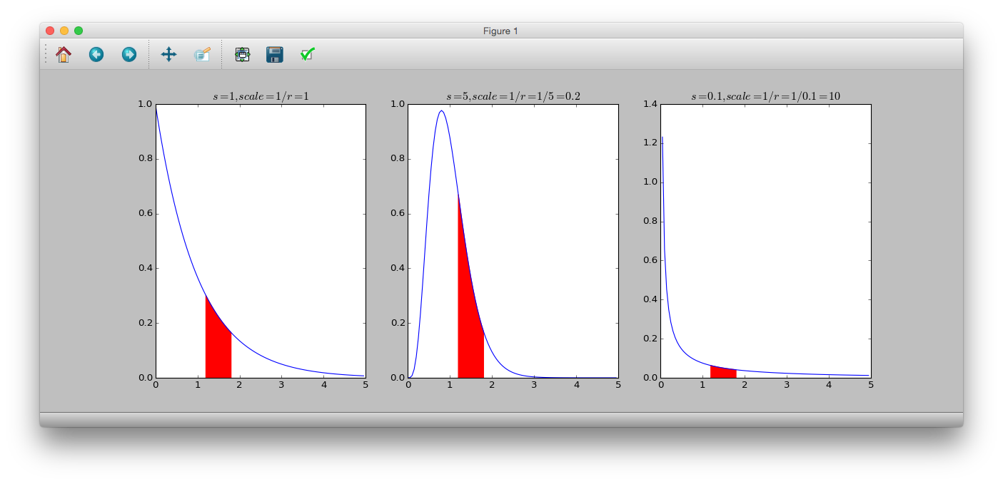
** Gamma distribution ** is a continuous probability distribution in which the range of random variables is 0 or more. The probability density function is.
p(y|s, r) = \frac{r^s}{\Gamma(s)}y^{s-1}\exp(-ry)
$ s $ is the shape parameter, $ r $ is the rate parameter, $ \ frac {1} {r} $ is the scale parameter, and $ \ Gamma (s) $ is the gamma function. The mean is $ \ frac {s} {r} $ and the variance is $ \ frac {s} {r ^ 2} $. Also, when $ s = 1 $, it becomes ** exponential distribution **.
# dgamma(y, shape, rate)
# 1/rate = scale
>>> y = numpy.arange(0, 5, 0.05)
>>> plt.subplot(131)
>>> plt.plot(y, sct.gamma.pdf(y, a=1, scale=1))
>>> plt.title('$s=1, scale=1/r=1$')
>>> plt.fill_between(numpy.arange(1.2, 1.8, 0.05), sct.gamma.pdf(numpy.arange(1.2, 1.8, 0.05), a=1, scale=1), color='r')
>>> plt.subplot(132)
>>> plt.plot(y, sct.gamma.pdf(y, a=5, scale=0.2))
>>> plt.title('$s=5, scale=1/r=1/5=0.2$')
>>> plt.fill_between(numpy.arange(1.2, 1.8, 0.05), sct.gamma.pdf(numpy.arange(1.2, 1.8, 0.05), a=5, scale=0.2), color='r')
>>> plt.subplot(133)
>>> plt.plot(y, sct.gamma.pdf(y, a=0.1, scale=10))
>>> plt.title('$s=0.1, scale=1/r=1/0.1=10$')
>>> plt.fill_between(numpy.arange(1.2, 1.8, 0.05), sct.gamma.pdf(numpy.arange(1.2, 1.8, 0.05), a=0.1, scale=10), color='r')
>>> plt.show()
Example: Relationship between leaf weight and flower weight of a fictitious plant
It seems that as $ x_i $ grows, so does $ y_i $.
\begin{eqnarray}
\mu_i &=& Ax_i^b \\
&=&\exp(a)x_i^b = \exp(a+b\log x_i) (\because A = \exp(a)) \\
\log\mu_i &=& a+blogx_i

\end{eqnarray}
>>> model = smf.glm('y ~ numpy.log(x)', data=d, family=sm.families.Gamma(link=sm.families.links.log))
>>> model.fit().summary()
                 Generalized Linear Model Regression Results
==============================================================================
Dep. Variable:                      y   No. Observations:                   50
Model:                            GLM   Df Residuals:                       48
Model Family:                   Gamma   Df Model:                            1
Link Function:                    log   Scale:                  0.325084605974
Method:                          IRLS   Log-Likelihood:                 58.471
Date:                Sat, 06 Jun 2015   Deviance:                       17.251
Time:                        20:38:39   Pearson chi2:                     15.6
No. Iterations:                    12
================================================================================
                   coef    std err          z      P>|z|      [95.0% Conf. Int.]
--------------------------------------------------------------------------------
Intercept       -1.0403      0.119     -8.759      0.000        -1.273    -0.808
numpy.log(x)     0.6832      0.068      9.992      0.000         0.549     0.817
================================================================================
get_y_mean = lambda b1, b2, x: numpy.exp(b1 + b2 * numpy.log(x))
model = smf.glm('y ~ numpy.log(x)', data=d, family=sm.families.Gamma(link=sm.families.links.log))
vc = model.fit().params

ax = plt.figure().add_subplot(111)
ax.plot(d.x, d.y, 'o')
ax.plot(d.x, get_y_mean(-1, 0.7, d.x),'--')
ax.plot(d.x, get_y_mean(vc[0], vc[1], d.x))


phi = model.fit().scale
m = get_y_mean(vc[0], vc[1], d.x)
scale = [(i * phi) for i in m]
shape = 1 / phi
def plot_pi(q):
    x = numpy.r_[numpy.array(d.x), numpy.array(d.x)[::-1]]
    y = numpy.r_[sct.gamma.ppf(q, a=shape, scale=scale), sct.gamma.ppf(1-q, a=shape, scale=scale)[::-1]]
    pair = [(x[i], y[i]) for i in range(len(x))]
    poly = plt.Polygon(pair, alpha=0.2, edgecolor='none')
    return poly
ax.add_patch(plot_pi(0.05))
ax.add_patch(plot_pi(0.25))

plt.show()

Recommended Posts