[PYTHON] [Introduction to minimize] Data analysis with SEIR model ♬

In preparation for data analysis of COVID-19, we will explain how to output the following graph. This figure is a figure in which the SEIR model of infectious disease is fitted to the given data using minimize @ scipy. SEIR_b6.88_ip1.22_gamma2.01_N762_E01_I00_R03.41_.png The method is almost as shown below. Both were helpful in many ways. 【reference】 (1) Beginning of mathematical model of infectious disease: Outline of SEIR model by Python and introduction to parameter estimation ② Mathematical prediction model for infectious diseases (SIR model): Case study (1) ③ I tried to predict the behavior of the new coronavirus with the SEIR model.

What i did

・ Code explanation ・ Try fitting with SIR model and SEIR model ・ Other models

・ Code explanation

The entire code is placed below. -Collive_particles / minimize_params.py I will leave the explanation to the above reference, and here I will explain the code used this time. The data was used from Reference (2). Also, for the minimize code, I referred to Reference ①. The Lib to be used is as follows. This time, it is implemented in the keras-gpu environment of the conda environment of Windows 10, but it is previously installed including scipy.

#include package
import numpy as np
from scipy.integrate import odeint
from scipy.optimize import minimize
import matplotlib.pyplot as plt

The differential equations of the SEIR model are defined below. Here, what to do with N will be decided as appropriate, but in this proposition, N = 763 people from the paper published in Reference (2), which was fixed. The differential equations of the SEIR model are as follows Here, in Reference (1), N is pushed into the variable beta, which is not explicitly expressed, but the following formula is easier to understand in terms of Uwan. The following is quoted from Reference ③.

{\begin{align}
\frac{dS}{dt} &= -\beta \frac{SI}{N} \\
\frac{dE}{dt} &=  \beta \frac{SI}{N}  -\epsilon E \\
\frac{dI}{dt} &=  \epsilon E -\gamma I \\
\frac{dR}{dt} &=  \gamma I \\
\end{align} 
}

If you look at the following while looking at the above, you can understand it because it is just right.

#define differencial equation of seir model
def seir_eq(v,t,beta,lp,ip):
    N=763
    a = -beta*v[0]*v[2]/N
    b = beta*v[0]*v[2]/N-(1/lp)*v[1]
    c = (1/lp)*v[1]-(1/ip)*v[2]
    d = (1/ip)*v[2]
    return [a,b,c,d]

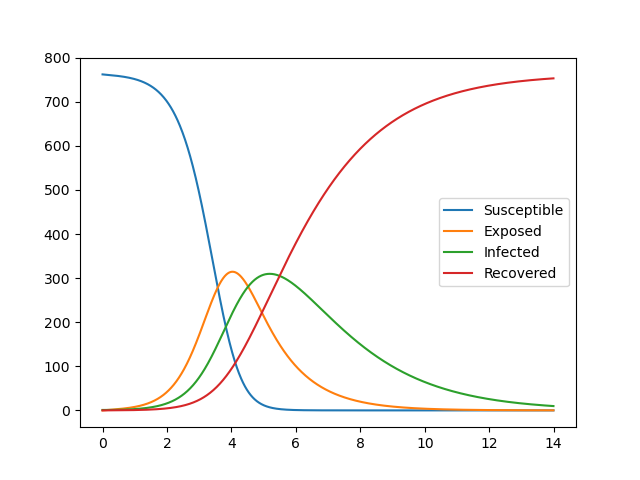
First, a solution is obtained based on the initial value as an ordinary differential equation.

#solve seir model
N,S0,E0,I0=762,0,1,0
ini_state=[N,S0,E0,I0]
beta,lp,ip=6.87636378, 1.21965986, 2.01373496 #2.493913  , 0.95107715, 1.55007883
t_max=14
dt=0.01
t=np.arange(0,t_max,dt)
plt.plot(t,odeint(seir_eq,ini_state,t,args=(beta,lp,ip))) #0.0001,1,3
plt.legend(['Susceptible','Exposed','Infected','Recovered'])
plt.pause(1)
plt.close()

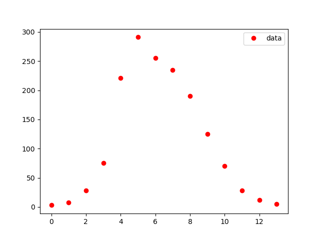
The result is as follows. If the parameters are estimated and changed here, most fittings can be performed, but complicated ones are difficult. As shown in Reference (2), substitute the data and output it to the graph as shown below.

#show observed i
#obs_i=np.loadtxt('fitting.csv')
data_influ=[3,8,28,75,221,291,255,235,190,125,70,28,12,5]
data_day = [1,2,3,4,5,6,7,8,9,10,11,12,13,14]
obs_i = data_influ

plt.plot(obs_i,"o", color="red",label = "data")
plt.legend()
plt.pause(1)
plt.close()

The result is as follows, and since this is an output for confirmation on the way, headings etc. are omitted. Now, the next is the estimation part. This evaluation function calculates with a differential equation using the value of the argument and returns the evaluation result.

#function which estimate i from seir model func 
def estimate_i(ini_state,beta,lp,ip):
    v=odeint(seir_eq,ini_state,t,args=(beta,lp,ip))
    est=v[0:int(t_max/dt):int(1/dt)]
    return est[:,2]

The log-likelihood function is defined as follows.

Refer to reference ① Basically, the problem is to change the parameters to find the maximum value of this log-likelihood function. (Actually, we take a minus and make it a minimization problem)
Here, the absolute value is taken to prevent the log argument from becoming negative.

#define logscale likelihood function
def y(params):
    est_i=estimate_i(ini_state,params[0],params[1],params[2])
    return np.sum(est_i-obs_i*np.log(np.abs(est_i)))

Use the following Scipy minimize function to find the maximum value.

#optimize logscale likelihood function
mnmz=minimize(y,[beta,lp,ip],method="nelder-mead")
print(mnmz)

The output is as follows

>python minimize_params.py
 final_simplex: (array([[6.87640764, 1.21966435, 2.01373196],
       [6.87636378, 1.21965986, 2.01373496],
       [6.87638203, 1.2196629 , 2.01372646],
       [6.87631916, 1.21964456, 2.0137297 ]]), array([-6429.40676091, -6429.40676091, -6429.40676091, -6429.4067609 ]))
           fun: -6429.406760912483
       message: 'Optimization terminated successfully.'
          nfev: 91
           nit: 49
        status: 0
       success: True
             x: array([6.87640764, 1.21966435, 2.01373196])

Take out beta_const, lp, gamma_const from the calculation result as follows, and calculate R0 below. This is the basic reproduction number, which is a guideline for the spread of infection. If R0 <1, it does not spread, but if R0> 1, it spreads and is an index showing the degree.

#R0
beta_const,lp,gamma_const = mnmz.x[0],mnmz.x[1],mnmz.x[2] #Infection rate, infection waiting time, removal rate (recovery rate)
print(beta_const,lp,gamma_const)
R0 = beta_const*(1/gamma_const)
print(R0)

This time, it is as follows, and since R0 = 3.41, the infection has spread.

6.876407637532918 1.2196643491443309 2.0137319643699927
3.4147581501415165

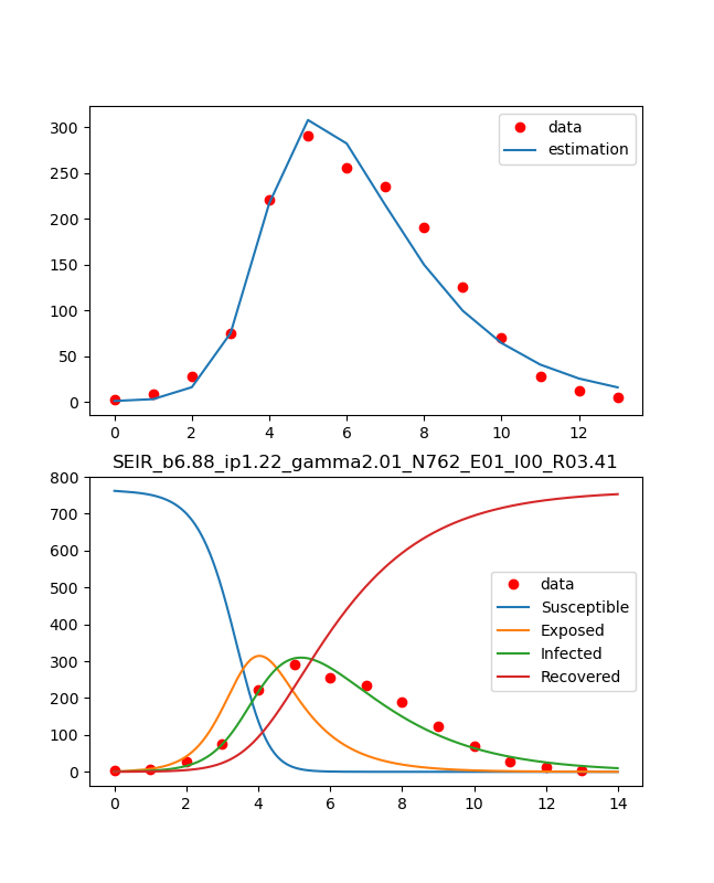
The obtained result is displayed on the graph.

#plot reult with observed data
fig, (ax1,ax2) = plt.subplots(2,1,figsize=(1.6180 * 4, 4*2))
lns1=ax1.plot(obs_i,"o", color="red",label = "data")
lns2=ax1.plot(estimate_i(ini_state,mnmz.x[0],mnmz.x[1],mnmz.x[2]), label = "estimation")
lns_ax1 = lns1+lns2
labs_ax1 = [l.get_label() for l in lns_ax1]
ax1.legend(lns_ax1, labs_ax1, loc=0)

lns3=ax2.plot(obs_i,"o", color="red",label = "data")
lns4=ax2.plot(t,odeint(seir_eq,ini_state,t,args=(mnmz.x[0],mnmz.x[1],mnmz.x[2])))
ax2.legend(['data','Susceptible','Exposed','Infected','Recovered'], loc=0)
ax2.set_title('SEIR_b{:.2f}_ip{:.2f}_gamma{:.2f}_N{:d}_E0{:d}_I0{:d}_R0{:.2f}'.format(beta_const,lp,gamma_const,N,E0,I0,R0))
plt.savefig('./fig/SEIR_b{:.2f}_ip{:.2f}_gamma{:.2f}_N{:d}_E0{:d}_I0{:d}_R0{:.2f}_.png'.format(beta_const,lp,gamma_const,N,E0,I0,R0)) 
plt.show()
plt.close()

The result is as above.

・ Other models

When I was doing this calculation, I found a slightly simpler SIR model and a slightly more complicated model, so I will summarize them. The SIR model is as follows because it is a model that ignores Exposed from S-E-I-R.

{\begin{align}
\frac{dS}{dt} &= -\beta \frac{SI}{N} \\
\frac{dI}{dt} &=  \beta \frac{SI}{N} -\gamma I \\
\frac{dR}{dt} &=  \gamma I \\
\end{align} 
}

You can understand the meaning of $ R_0 $ by rewriting as follows.

{\begin{align}
\frac{dS}{dt} &= -R_0 \frac{S}{N} \frac{dR}{dt} \\
R_0 &= \frac{\beta}{\gamma}\\ 
\frac{dI}{dt} &= 0 \Infected person peak at\\
R_0 &=  \frac{\beta}{\gamma}=  \frac{N}{S_0} \\
\end{align} 
}

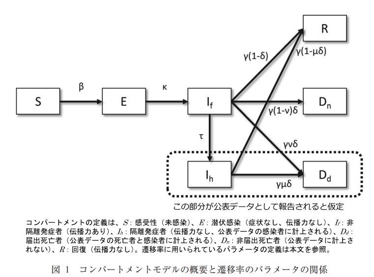
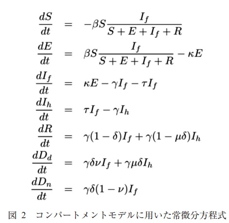
On the other hand, in a complicated situation such as a transition of death and death without notification, it will be as follows. It is assumed that deaths do not contribute to infection.

COVID-19 may look like this The figure is from the following document in Reference ① ・ Analysis of epidemics of Ebola virus infection using a mathematical model

Summary

-Data fitting can now be done automatically by minimize @ scipy. ・ I was able to fit the actual data with the SEIR model.

・ Next time, I would like to analyze the data of each country of COVID-19.