Overview

Using the Titanic data that is often used at the beginning of kaggle, I tried factor analysis. However, this time, it was not done for the purpose of prediction. The purpose was to observe the characteristics of the data simply by using the statistical analysis method. So, I decided to perform factor analysis on the train / test data.

I am writing an article on principal component analysis using the same data as this article. I wrote this article as a sequel. The programs (1.-4.) Up to the pre-processing in the following [Analysis_Details] are "almost" the same. (Please check [Analysis_Summary] below.) https://qiita.com/cleeeear/items/67210d977a901ebf9b4f

Premise

――What is factor analysis? Consider expressing the explanatory variables as "linear combinations of common factors and unique factors".

X=FA+UB

$ X: Data (number of data (N) x number of explanatory variables (n)) $ $ F: Common factor matrix (N x number of factors (m)) $

Consists of common factors (column vectors) in which each explanatory variable is commonly involved. $ A: Factor loading (of common factors) $ (m x n) $
When referring to "factor loading" below, this refers to this. $ U: Intrinsic factor matrix (N × n) $
Each explanatory variable consists of a separate eigenfactor (column vector). $ B: Factor loading of eigenfactor (N × n) $
Diagonal matrix

(Each element $ a_ {ij} $ of factor loading A is Under the following analysis conditions (1) and (2), which is also the analysis of this article, It is a correlation value between the common factor $ F_ {i} $ and the explanatory variable $ X_ {i} $.

① Common factor: Orthogonal factor (2) Explanatory variable: Standardized and used (mean 0 variance 1) )

In the factor analysis, this factor loading amount A is obtained. By grasping the characteristics of common factors from the obtained factor loading Common factors are often used as a summary of data.

Analysis_Overview

--Analytical data Titanic data (train + test). You can download it from the following (kaggle). (However, you need to sign in to kaggle.) https://www.kaggle.com/c/titanic/data --Settings in this analysis --Common factors: 2 & orthogonal factors --Explanatory variable: Standardized and used (mean 0 variance 1)

confirmation point --Factor loading --Variables to be excluded in the analysis This time, for simple analysis, the following variables, which are difficult to preprocess, are excluded from the analysis.
Cabin
Ticket
Name
Embarked_C
Embarked_Q
Embarked_S

Analysis_Details

Library import

import os
import pandas as pd
import matplotlib.pyplot as plt
from IPython.display import display
from sklearn.decomposition import PCA

Variable definition (titanic data csv storage destination, etc.)

Premise code that stores Titanic data csv (train.csv, test.csv) in the folder "data".

#Current folder
forlder_cur = os.getcwd()
print(" forlder_cur : {}".format(forlder_cur))
print(" isdir:{}".format(os.path.isdir(forlder_cur)))

#data storage location
folder_data = os.path.join(forlder_cur , "data")
print(" folder_data : {}".format(folder_data))
print(" isdir:{}".format(os.path.isdir(folder_data)))

#data file

## train.csv
fpath_train = os.path.join(folder_data , "train.csv")
print(" fpath_train : {}".format(fpath_train))
print(" isdir:{}".format(os.path.isfile(fpath_train)))

## test.csv
fpath_test = os.path.join(folder_data , "test.csv")
print(" fpath_test : {}".format(fpath_test))
print(" isdir:{}".format(os.path.isfile(fpath_test)))

# id
id_col = "PassengerId"

#Objective variable
target_col = "Survived"

Import Titanic data The data "all_data" (train + test) created by the code below will be used later.

# train.csv
train_data = pd.read_csv(fpath_train)
print("train_data :")
print("n = {}".format(len(train_data)))
display(train_data.head())

# test.csv
test_data = pd.read_csv(fpath_test)
print("test_data :")
print("n = {}".format(len(test_data)))
display(test_data.head())

# train_and_test
col_list = list(train_data.columns)
tmp_test = test_data.assign(Survived=None)
tmp_test = tmp_test[col_list].copy()
print("tmp_test :")
print("n = {}".format(len(tmp_test)))
display(tmp_test.head())

all_data = pd.concat([train_data , tmp_test] , axis=0)
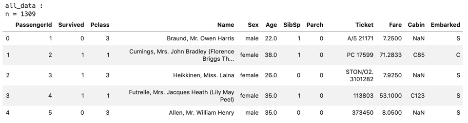
print("all_data :")
print("n = {}".format(len(all_data)))
display(all_data.head())

Pretreatment Dummy variable conversion, missing completion, and variable deletion are performed for each variable, and the created data "proc_all_data" is used later.

#copy
proc_all_data = all_data.copy()

# Sex -------------------------------------------------------------------------
col = "Sex"

def app_sex(x):
    if x == "male":
        return 1
    elif x == 'female':
        return 0
    #Missing
    else:
        return 0.5
proc_all_data[col] = proc_all_data[col].apply(app_sex)

print("columns:{}".format(col) , "-" * 40)
display(all_data[col].value_counts())
display(proc_all_data[col].value_counts())
print("n of missing :" , len(proc_all_data.query("{0} != {0}".format(col))))

# Age -------------------------------------------------------------------------
col = "Age"

medi = proc_all_data[col].median()
proc_all_data[col] = proc_all_data[col].fillna(medi)

print("columns:{}".format(col) , "-" * 40)
display(all_data[col].value_counts())
display(proc_all_data[col].value_counts())
print("n of missing :" , len(proc_all_data.query("{0} != {0}".format(col))))
print("median :" , medi)

# Fare -------------------------------------------------------------------------
col = "Fare"

medi = proc_all_data[col].median()
proc_all_data[col] = proc_all_data[col].fillna(medi)

print("columns:{}".format(col) , "-" * 40)
display(all_data[col].value_counts())
display(proc_all_data[col].value_counts())
print("n of missing :" , len(proc_all_data.query("{0} != {0}".format(col))))
print("median :" , medi)

# Embarked -------------------------------------------------------------------------
col = "Embarked"

proc_all_data = pd.get_dummies(proc_all_data , columns=[col])

print("columns:{}".format(col) , "-" * 40)
display(all_data.head())
display(proc_all_data.head())

# Cabin -------------------------------------------------------------------------
col = "Cabin"

proc_all_data = proc_all_data.drop(columns=[col])

print("columns:{}".format(col) , "-" * 40)
display(all_data.head())
display(proc_all_data.head())

# Ticket -------------------------------------------------------------------------
col = "Ticket"

proc_all_data = proc_all_data.drop(columns=[col])

print("columns:{}".format(col) , "-" * 40)
display(all_data.head())
display(proc_all_data.head())

# Name -------------------------------------------------------------------------
col = "Name"

proc_all_data = proc_all_data.drop(columns=[col])

print("columns:{}".format(col) , "-" * 40)
display(all_data.head())
display(proc_all_data.head())

# Embarked_C -------------------------------------------------------------------------
col = "Embarked_C"

proc_all_data = proc_all_data.drop(columns=[col])

print("columns:{}".format(col) , "-" * 40)
display(all_data.head())
display(proc_all_data.head())

# Embarked_Q -------------------------------------------------------------------------
col = "Embarked_Q"

proc_all_data = proc_all_data.drop(columns=[col])

print("columns:{}".format(col) , "-" * 40)
display(all_data.head())
display(proc_all_data.head())

# Embarked_S -------------------------------------------------------------------------
col = "Embarked_S"

proc_all_data = proc_all_data.drop(columns=[col])

print("columns:{}".format(col) , "-" * 40)
display(all_data.head())
display(proc_all_data.head())

proc_all_data :

Factor analysis 5-1. Standardization, fit After standardizing the explanatory variables, perform factor analysis.

#Explanatory variable
feature_cols = list(set(proc_all_data.columns) - set([target_col]) - set([id_col]))
print("feature_cols :" , feature_cols)
print("len of feature_cols :" , len(feature_cols))

features_tmp = proc_all_data[feature_cols]
print("features(Before standardization):")
display(features_tmp.head())

#Standardization
ss = StandardScaler()
features = pd.DataFrame(
    ss.fit_transform(features_tmp)
    , columns=feature_cols
)
print("features(After standardization):")
display(features.head())

features (before and after standardization):

5-2. Factor loading matrix

#Factor analysis
n_components = 2
fact_analysis = FactorAnalysis(n_components=n_components)
fact_analysis.fit(features)

#Factor loading matrix(X = FA +UB A)
print("Factor loading matrix(X = FA +UB A) :")
components_df = pd.DataFrame(
    fact_analysis.components_
    ,columns=feature_cols
)
display(components_df)

components_df:

5-3. [Reference] ① Factor matrix ② Correlation between factors ③ "Correlation between factor loading matrix (A) --factor (F) and explanatory variable (X)" This is output for reference. Regarding (2), confirm that it is an orthogonal factor. About ③ This time, the explanatory variables are standardized and orthogonal factors, so (Although there is an error because it is an approximate solution) Confirm that the difference is 0.

#factor
print("Factor matrix(X = FA +UB F) :")
fact_columns = ["factor_{}".format(i+1) for i in range(n_components)]
factor_df = pd.DataFrame(
    fact_analysis.transform(features)
    , columns=fact_columns
)
display(factor_df)

#Correlation between factors
corr_fact_df = factor_df.corr()
print("Correlation between factors:")
display(corr_fact_df)

#Correlation between factors(Decimal notation)
def show_float(x):
    return "{:.5f}".format(x)
print("* Decimal notation:")
display(corr_fact_df.applymap(show_float))

# [Factor loading matrix(A)] - [factor(F)And explanatory variables(X)Correlation of]
##factor(F)And explanatory variables(X)Correlation of
fact_exp_corr_df = pd.DataFrame()
for exp_col in feature_cols:
    data = list()
    for fact_col in fact_columns:
        x = features[exp_col]
        f = factor_df[fact_col]
        data.append(x.corr(f))
    fact_exp_corr_df[exp_col] = data
print("factor(F)And explanatory variables(X)Correlation of:")
display(fact_exp_corr_df)

print("[Factor loading matrix(A)] - [factor(F)And explanatory variables(X)Correlation of]:")
display(components_df - fact_exp_corr_df)

5-4. Graphing _1 / 2 (Check factor loading for each factor)

#Graphing(Bar / line graph_Factor loading of each factor)
for i in range(len(fact_columns)):
    #Load of target factor
    fact_col = fact_columns[i]
    component = components_df.iloc[i]
    #Load amount and its absolute value, absolute value rank
    df = pd.DataFrame({
        "component":component
        , "abs_component":component.abs()
    })
    df["rank_component"] = df["abs_component"].rank(ascending=False)
    df.sort_values(by="rank_component" , inplace=True)
    print("[{}]".format(fact_col) , "-" * 80)
    display(df)
    
    #Graphing(Bar graph: Factor loading, Line: Absolute value)
    x_ticks = df.index.tolist()
    x_ticks_num = [i for i in range(len(x_ticks))]
    fig = plt.figure(figsize=(12 , 5))
    plt.bar(x_ticks_num , df["component"] , label="factor loadings" , color="c")
    plt.plot(x_ticks_num , df["abs_component"] , label="[abs] factor loadings" , color="r" , marker="o")
    plt.legend()
    plt.xticks(x_ticks_num , labels=x_ticks)
    plt.xlabel("features")
    plt.ylabel("factor loadings")
    plt.show()
    
    fig.savefig("bar_{}.png ".format(fact_col))

5-5. Graphing_2 / 2 (Plot factor loadings on two axes consisting of both factors)

#Graphing(Factor loading of two factors)

#Graph display function
def plotting_fact_load_of_2_fact(x_fact , y_fact):
    #Data frame for graph
    df = pd.DataFrame({
        x_fact : components_df.iloc[0].tolist()
        , y_fact : components_df.iloc[1].tolist()    
        }
        ,index = components_df.columns
    )

    fig = plt.figure(figsize=(10 , 10))
    for exp_col in df.index.tolist():
        data = df.loc[exp_col]
        x_label = df.columns.tolist()[0]
        y_label = df.columns.tolist()[1]
        x = data[x_label]
        y = data[y_label]
        plt.plot(x
                 , y
                 , label=exp_col
                 , marker="o"
                 , color="r")
        plt.annotate(exp_col , xy=(x , y))
    plt.xlabel(x_label)
    plt.ylabel(y_label)
    plt.grid()
    
    print("x = [{x_fact}] , y = [{y_fact}]".format(
        x_fact=x_fact
        , y_fact=y_fact
    ) , "-" * 80)
    display(df)
    plt.show()
    fig.savefig("plot_{x_fact}_{y_fact}.png ".format(
        x_fact=x_fact
        , y_fact=y_fact
    ))

#graph display
plotting_fact_load_of_2_fact("factor_1" , "factor_2")

As a premise, the range of Pclass (passenger class) is 1 to 3, and it seems that the smaller the range, the higher the class.

About the first factor The factor load of Fare (boarding fee) is large, and the Pclass (passenger class) is small. (That is, the higher the class, the greater the factor load) So the first factor is "Indicator to evaluate wealth" It seems that you can think of it.

It is an index similar to the first principal component in the principal component analysis described above.

About the second factor As absolute values, Parch (number of parents and children) and SibSp (number of siblings and spouses) are both large and positive. So the second factor is "Indicator of family size" It seems that you can think of it.

Summary

As a result of factor analysis with two factors As the first factor, "an index to evaluate wealth" And as the second factor, "an index showing the number of families" was gotten.

The first factor is "First principal component of the previous principal component analysis" It became an index similar to. In a book on multivariate analysis It was stated that the essence of principal component analysis and factor analysis is the same, It is a feeling that the result clearly shows that.

[PYTHON] I tried factor analysis with Titanic data!

Overview

Premise

Analysis_Overview

Analysis_Details

Summary