[PYTHON] I tried principal component analysis with Titanic data!
Overview
Using the Titanic data that is often used at the beginning of kaggle, I tried principal component analysis. However, this time, it was not done for the purpose of prediction. The purpose was to observe the characteristics of the data simply by using the statistical analysis method. So, I decided to analyze the principal components of the train / test data together.
Premise
――What is principal component analysis?
For data represented by multiple axes (variables)
A method to find "axis with high data variation".
Because of dimensional compression when predicting
When analyzing existing data, it is often done for summarization.
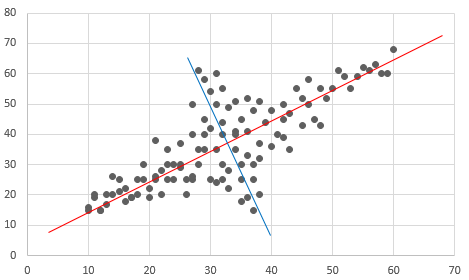
In the figure below (image)
The red axis has the highest variation, followed by the blue axis (orthogonal to the red axis) with the highest variation.
Principal component analysis finds such red and blue axes.
Analysis_Overview
--Analytical data Titanic data (train + test). You can download it from the following (kaggle). (However, you need to sign in to kaggle.) https://www.kaggle.com/c/titanic/data
- confirmation point --Contribution rate --Eigenvector --Factor loading --Variables to be excluded in the analysis This time, for simple analysis, the following variables, which are difficult to preprocess, are excluded from the analysis.
- Cabin
- Ticket
- Name
Analysis_Details
- Library import
import os
import pandas as pd
import matplotlib.pyplot as plt
from IPython.display import display
from sklearn.decomposition import PCA
- Variable definition (titanic data csv storage destination, etc.)
- Premise code that stores Titanic data csv (train.csv, test.csv) in the folder "data".
#Current folder
forlder_cur = os.getcwd()
print(" forlder_cur : {}".format(forlder_cur))
print(" isdir:{}".format(os.path.isdir(forlder_cur)))

#data storage location
folder_data = os.path.join(forlder_cur , "data")
print(" folder_data : {}".format(folder_data))
print(" isdir:{}".format(os.path.isdir(folder_data)))

#data file

## train.csv
fpath_train = os.path.join(folder_data , "train.csv")
print(" fpath_train : {}".format(fpath_train))
print(" isdir:{}".format(os.path.isfile(fpath_train)))

## test.csv
fpath_test = os.path.join(folder_data , "test.csv")
print(" fpath_test : {}".format(fpath_test))
print(" isdir:{}".format(os.path.isfile(fpath_test)))

# id
id_col = "PassengerId"

#Objective variable
target_col = "Survived"
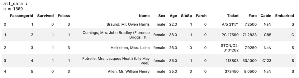
- Import Titanic data The data "all_data" (train + test) created by the code below will be used later.
# train.csv
train_data = pd.read_csv(fpath_train)
print("train_data :")
print("n = {}".format(len(train_data)))
display(train_data.head())

# test.csv
test_data = pd.read_csv(fpath_test)
print("test_data :")
print("n = {}".format(len(test_data)))
display(test_data.head())

# train_and_test
col_list = list(train_data.columns)
tmp_test = test_data.assign(Survived=None)
tmp_test = tmp_test[col_list].copy()
print("tmp_test :")
print("n = {}".format(len(tmp_test)))
display(tmp_test.head())

all_data = pd.concat([train_data , tmp_test] , axis=0)
print("all_data :")
print("n = {}".format(len(all_data)))
display(all_data.head())
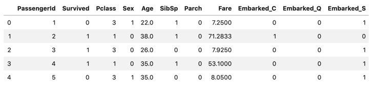
- Pretreatment Dummy variable conversion, missing completion, and variable deletion are performed for each variable, and the created data "proc_all_data" is used later.
#copy
proc_all_data = all_data.copy()

# Sex -------------------------------------------------------------------------
col = "Sex"

def app_sex(x):
    if x == "male":
        return 1
    elif x == 'female':
        return 0
    #Missing
    else:
        return 0.5
proc_all_data[col] = proc_all_data[col].apply(app_sex)

print("columns:{}".format(col) , "-" * 40)
display(all_data[col].value_counts())
display(proc_all_data[col].value_counts())
print("n of missing :" , len(proc_all_data.query("{0} != {0}".format(col))))

# Age -------------------------------------------------------------------------
col = "Age"

medi = proc_all_data[col].median()
proc_all_data[col] = proc_all_data[col].fillna(medi)

print("columns:{}".format(col) , "-" * 40)
display(all_data[col].value_counts())
display(proc_all_data[col].value_counts())
print("n of missing :" , len(proc_all_data.query("{0} != {0}".format(col))))
print("median :" , medi)

# Fare -------------------------------------------------------------------------
col = "Fare"

medi = proc_all_data[col].median()
proc_all_data[col] = proc_all_data[col].fillna(medi)

print("columns:{}".format(col) , "-" * 40)
display(all_data[col].value_counts())
display(proc_all_data[col].value_counts())
print("n of missing :" , len(proc_all_data.query("{0} != {0}".format(col))))
print("median :" , medi)

# Embarked -------------------------------------------------------------------------
col = "Embarked"

proc_all_data = pd.get_dummies(proc_all_data , columns=[col])

print("columns:{}".format(col) , "-" * 40)
display(all_data.head())
display(proc_all_data.head())

# Cabin -------------------------------------------------------------------------
col = "Cabin"

proc_all_data = proc_all_data.drop(columns=[col])

print("columns:{}".format(col) , "-" * 40)
display(all_data.head())
display(proc_all_data.head())

# Ticket -------------------------------------------------------------------------
col = "Ticket"

proc_all_data = proc_all_data.drop(columns=[col])

print("columns:{}".format(col) , "-" * 40)
display(all_data.head())
display(proc_all_data.head())

# Name -------------------------------------------------------------------------
col = "Name"

proc_all_data = proc_all_data.drop(columns=[col])

print("columns:{}".format(col) , "-" * 40)
display(all_data.head())
display(proc_all_data.head())
proc_all_data :
- Principal component analysis (calculation of contribution rate)
#Explanatory variable
feature_cols = list(set(proc_all_data.columns) - set([target_col]) - set([id_col]))
print("feature_cols :" , feature_cols)
print("len of feature_cols :" , len(feature_cols))

features = proc_all_data[feature_cols]

pca = PCA()
pca.fit(features)

print("Number of main components: " , pca.n_components_)
print("Contribution rate: " , ["{:.2f}".format(ratio) for ratio in pca.explained_variance_ratio_])
As shown in the results below, the first principal component is overwhelmingly highly variable.
In the following, the eigenvector of the first principal component and the factor loading are confirmed.

- Eigenvector of the first principal component
6-1. Data transformation
#Eigenvector(First main component)

components_df = pd.DataFrame({
    "feature":feature_cols
    , "component":pca.components_[0]
})
components_df["abs_component"] = components_df["component"].abs()
components_df["rank_component"] = components_df["abs_component"].rank(ascending=False)

#Descending sort by absolute value of vector value
components_df.sort_values(by="abs_component" , ascending=False , inplace=True)
display(components_df)
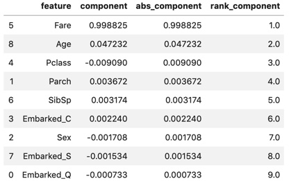
components_df :
6-2. Graphing
#Graph creation
max_abs_component = max(components_df["abs_component"])
min_component = min(components_df["component"])
x_ticks_num = list(i for i in range(len(components_df)))
fig = plt.figure(figsize=(15,8))
plt.grid()
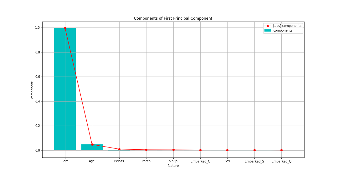
plt.title("Components of First Principal Component")
plt.xlabel("feature")
plt.ylabel("component")
plt.xticks(ticks=x_ticks_num , labels=components_df["feature"])
plt.bar(x_ticks_num , components_df["component"] , color="c" , label="components")
plt.plot(x_ticks_num , components_df["abs_component"] , color="r" , marker="o" , label="[abs] components")
plt.legend()
plt.show()
Fare (boarding fee) is overwhelmingly large, followed by Age (age). There are only a few others.
Looking only at the eigenvectors, it seems to be the principal component summarized by Fare.
However, since the value of the eigenvector changes depending on the size of the variance of the target variable,
Let's look at the factor loading that will be calculated later.
- Factor loading of the first main component
7-1. Data transformation
#Main component score(First main component)
score = pca.transform(features)[: , 0]
#Factor loading
dict_fact_load = dict()
for col in feature_cols:
data = features[col]
factor_loading = data.corr(pd.Series(score))
dict_fact_load[col] = factor_loading
fact_load_df = pd.DataFrame({
"feature":feature_cols
, "factor_loading":[dict_fact_load[col] for col in feature_cols]
})
fact_load_df["abs_factor_loading"] = fact_load_df["factor_loading"].abs()
fact_load_df["rank_factor_loading"] = fact_load_df["abs_factor_loading"].rank(ascending=False)
#Descending sort by absolute value of vector value
fact_load_df.sort_values(by="abs_factor_loading" , ascending=False , inplace=True)
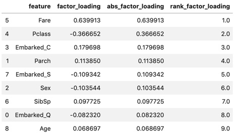
display(fact_load_df)
7-2. Graphing
#Graph creation
max_abs_factor_loading = max(fact_load_df["abs_factor_loading"])
min_factor_loading = min(fact_load_df["factor_loading"])
x_ticks_num = list(i for i in range(len(fact_load_df)))
plt.figure(figsize=(15,8))
plt.grid()
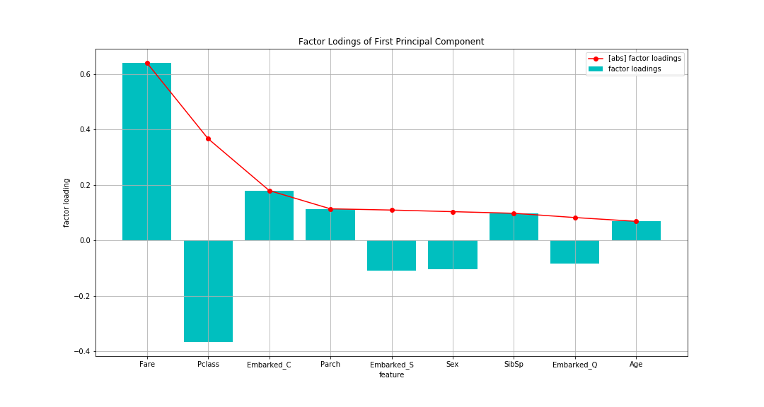
plt.title("Factor Lodings of First Principal Component")
plt.xlabel("feature")
plt.ylabel("factor loading")
plt.xticks(ticks=x_ticks_num , labels=fact_load_df["feature"])
plt.bar(x_ticks_num , fact_load_df["factor_loading"] , color="c" , label="factor loadings")
plt.plot(x_ticks_num , fact_load_df["abs_factor_loading"] , color="r" , marker="o" , label="[abs] factor loadings")
plt.legend()
plt.show()
Looking at the factor loading, As an absolute value (line), Fare (boarding fare) is the highest, followed by Pclass (passenger class). With a difference in Pclass, the others are about as small. The first main component is "Indicator to evaluate wealth" It seems that you can think of it.
Compared to the eigenvectors confirmed above Regarding Fare, the eigenvector was overwhelmingly the largest, but the factor loading did not make such a difference. Regarding Age, it was the second largest in the eigenvector, but the lowest in the factor loading. Fare and Age seem to be highly dispersed.
If you try to judge the correlation between the principal component score and each variable from the eigenvector,
I was about to make a mistake.
Factor loading should be calculated and confirmed.
Summary
As a result of principal component analysis "Evaluate wealth" index is obtained, The index was the one that most customers (each data) could be divided (variated).
We also found that the eigenvectors and factor loadings have different tendencies. this is, "(To check the contents of the main component) When looking at the correlation between the principal components and each variable, look at the factor loading. Judging only by the eigenvectors (Because it is affected by the size of the variance) May be misleading " There is a caveat.
Recommended Posts