[PYTHON] [Introduction to matplotlib] Read the end time from COVID-19 data ♬
There are some things that I learned from the previous simulation of the new corona, but if you look closely, it makes me think that the peak of infection may be predictable from the graph of the infection status of corona.
It was the following simulation.
 That is, the red bar graph shows the number of infections, and the green bar graph shows the number of infections, but it is difficult to predict how much the number of infections will increase, but at least the number of infections is limited by the number of infections. It does not exceed the number. Moreover, when expressed in terms of cure rate, it is almost 100% at the end. Moreover, the cure rate always peaks later than the peak of infection. At first glance, it seems that the number of infections that peak first is easier to determine the end, but it is not clear whether this peak is necessarily the upper limit.
On the other hand, the number of cures peaks around 50% and is expected to gradually approach that value.
In other words, if you follow this value, it seems that the end time will be roughly visible.
Looking at the graph above with the belief that the infection is becoming saturated from the beginning of healing.
This time, let's first see if the actual data behaves in the same way.
【reference】
・ Visualize the number of people infected with coronavirus with matplotlib
That is, the red bar graph shows the number of infections, and the green bar graph shows the number of infections, but it is difficult to predict how much the number of infections will increase, but at least the number of infections is limited by the number of infections. It does not exceed the number. Moreover, when expressed in terms of cure rate, it is almost 100% at the end. Moreover, the cure rate always peaks later than the peak of infection. At first glance, it seems that the number of infections that peak first is easier to determine the end, but it is not clear whether this peak is necessarily the upper limit.
On the other hand, the number of cures peaks around 50% and is expected to gradually approach that value.
In other words, if you follow this value, it seems that the end time will be roughly visible.
Looking at the graph above with the belief that the infection is becoming saturated from the beginning of healing.
This time, let's first see if the actual data behaves in the same way.
【reference】
・ Visualize the number of people infected with coronavirus with matplotlib
What i did
・ Code explanation ・ Visualize the number of infected people in each country
・ Code explanation
The code is below. ・ Collive_particles / draw_covid19.py
This time, it is a visualization method of multiple data. For visualization of infection data, obtain at least 3 data from the following sites. For the sake of simplicity, I downloaded the zip file from the following reference site and unzipped it. (The link below is the link page of the file. We recommend batch download from the reference below) time_series_19-covid-Confirmed.csv time_series_19-covid-Deaths.csv time_series_19-covid-Recovered.csv 【reference】 ・ CSSEGISandData / COVID-19 We will process these data appropriately and draw a graph similar to the above. The graph drawing is explained below. First, use the following Lib. Here, again, Jetson-nano is used as the environment, but pandas is newly installed. As for reference, I got an error if it was simple, so I finally entered it with the following command.
sudo apt-get install python-pandas
sudo apt-get install python3-pandas
The following code worked with python, but import pandas didn't work with python3.
- It seems to work as follows? ??
$ python3
Python 3.6.9 (default, Nov  7 2019, 10:44:02)
[GCC 8.3.0] on linux
Type "help", "copyright", "credits" or "license" for more information.
>>> import pandas as pd
>>>
【reference】 ・ How to install Pandas in 3 minutes without using pip
# -*- coding: utf-8 -*-
import numpy as np
import matplotlib.pyplot as plt
import pandas as pd
Next, read the three csv files as follows.
#Read CSV data with pandas.
data = pd.read_csv('COVID-19/csse_covid_19_data/csse_covid_19_time_series/time_series_19-covid-Confirmed.csv')
data_r = pd.read_csv('COVID-19/csse_covid_19_data/csse_covid_19_time_series/time_series_19-covid-Recovered.csv')
data_d = pd.read_csv('COVID-19/csse_covid_19_data/csse_covid_19_time_series/time_series_19-covid-Deaths.csv')
Define the variable. The data to be read has the following structure, so the first four are excluded.
| Province/State | Country/Region | Lat | Long | 1/22/20 | 1/23/20 | 1/24/20 | 1/25/20 |
|---|---|---|---|---|---|---|---|
| Thailand | 15 | 101 | 2 | 3 | 5 | 7 | |
| Japan | 36 | 138 | 2 | 1 | 2 | 2 | |
| New South Wales | Australia | -33.8688 | 151.2093 | 0 | 0 | 0 | 0 |
The date has been changed to the number of days. .. .. From the above reference article
confirmed = [0] * (len(data.columns) - 4)
confirmed_r = [0] * (len(data_r.columns) - 4)
confirmed_d = [0] * (len(data_d.columns) - 4)
recovered_rate = [0] * (len(data_r.columns) - 4)
deaths_rate = [0] * (len(data_d.columns) - 4)
days_from_22_Jan_20 = np.arange(0, len(data.columns) - 4, 1)
This time we will look at the data of Wuhan.
city = "Hubei"
The first variable below is provided to store the total number of cases, total number of cures, and total number of deaths for title display. As you can see from the above data, it is lined up with states and countries, so to bring in Wuhan data, use ʻif (data.iloc [i] [0] == city): `. The country uses the commented out. Store the daily numbers in confirmed, confirmed_r, and confirmed_d. Since the number of cases data is a cumulative value, we subtract the number of cases of healing on that day and change it to the number of infections on that day. The + = calculation is used to obtain the total value of regions in the same country but in different regions.
#Process the data
t_cases = 0
t_recover = 0
t_deaths = 0
for i in range(0, len(data), 1):
    #if (data.iloc[i][1] == city): #for country/region
    if (data.iloc[i][0] == city):  #for province:/state
        print(str(data.iloc[i][0]) + " of " + data.iloc[i][1])
        for day in range(4, len(data.columns), 1):
            confirmed[day - 4] += data.iloc[i][day] -  data_r.iloc[i][day]
            confirmed_r[day - 4] += data_r.iloc[i][day]
            confirmed_d[day - 4] += data_d.iloc[i][day]
        t_recover += data_r.iloc[i][day]
        t_deaths += data_d.iloc[i][day]
This time, I want to see the end of the above, so I am calculating the cure rate. We also calculate the mortality rate of concern.
tl_confirmed = 0
for i in range(0, len(confirmed), 1):
    tl_confirmed = confirmed[i] + confirmed_r[i] + confirmed_d[i]
    if tl_confirmed > 0:
        recovered_rate[i]=float(confirmed_r[i]*100)/float(tl_confirmed)
        deaths_rate[i]=float(confirmed_d[i]*100)/float(tl_confirmed)
    else:
        continue
t_cases = tl_confirmed
It is graphed below. This time, multiple graphs can be displayed together.
- This article seems to be more versatile and nice. For reference, I think the following code is easy to understand. 【reference】 -Secondary axis with twinx (): how to add to legend?
#matplotlib drawing
fig, (ax1,ax2) = plt.subplots(2,1,figsize=(1.6180 * 4, 4*2))
ax3 = ax1.twinx()
ax4 = ax2.twinx()

lns1=ax1.plot(days_from_22_Jan_20, confirmed, "o-", color="red",label = "cases")
lns2=ax1.plot(days_from_22_Jan_20, confirmed_r, "*-", color="green",label = "recovered")
lns3=ax3.plot(days_from_22_Jan_20, confirmed_d, "D-", color="black", label = "deaths")
lns4=ax2.plot(days_from_22_Jan_20, recovered_rate, "*-", color="green",label = "recovered")
lns5=ax4.plot(days_from_22_Jan_20, deaths_rate, "D-", color="black", label = "deaths")

lns_ax1 = lns1+lns2+lns3
labs_ax1 = [l.get_label() for l in lns_ax1]
ax1.legend(lns_ax1, labs_ax1, loc=0)

lns_ax2 = lns4+lns5
labs_ax2 = [l.get_label() for l in lns_ax2]
ax2.legend(lns_ax2, labs_ax2, loc=0)

ax1.set_title(city +" ; {} cases, {} recovered, {} deaths".format(t_cases,t_recover,t_deaths))
ax1.set_xlabel("days from 22, Jan, 2020")
ax1.set_ylabel("casas, recovered ")
ax2.set_ylabel("recovered_rate %")
ax2.set_ylim(0,100)

ax3.set_ylabel("deaths ")
ax4.set_ylabel("deaths_rate %")
ax4.set_ylim(0,10)
ax1.grid()
ax2.grid()

plt.pause(1)
plt.savefig('./fig/fig_{}_.png'.format(city))
plt.close()
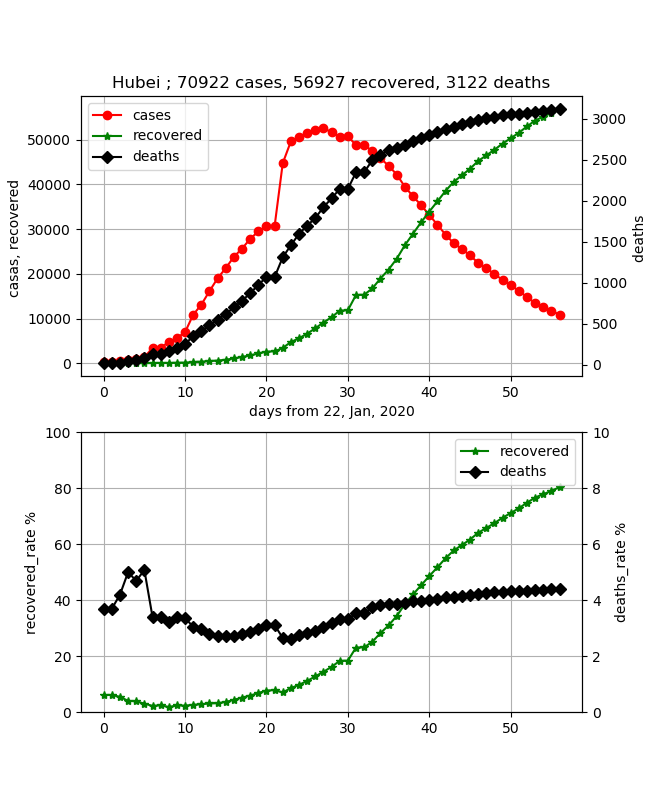
This data is quite good data to compare with the simulation. Unfortunately, the part that changed the counting method looks big. From this data, if this can be reproduced by simulation, it will be possible to simulate the transmission of infection in Wuhan this time. And if you look at the cure rate, you can see that 50% is the peak of this infection transmission, and it can be predicted that it will end in about the same number of days thereafter. In other words, it peaks about 40 days after the start of infection, and now, about 20 days after that, it is likely to end in about 20 days. In addition, the mortality rate is gradually increasing, and it seems to be about 4.5%. This does not increase the number of newly infected people, but I think it is unavoidable because the deaths will continue until the final night.
- I hope that the medical procedure will be improved and you will not die gradually.
・ Visualize the number of infected people in each country
Let's output the situation of the country you care about Below, I wrote various comments, but I'm not sure because it is just an impression of amateur Uwan looking at the graph.
·Korea
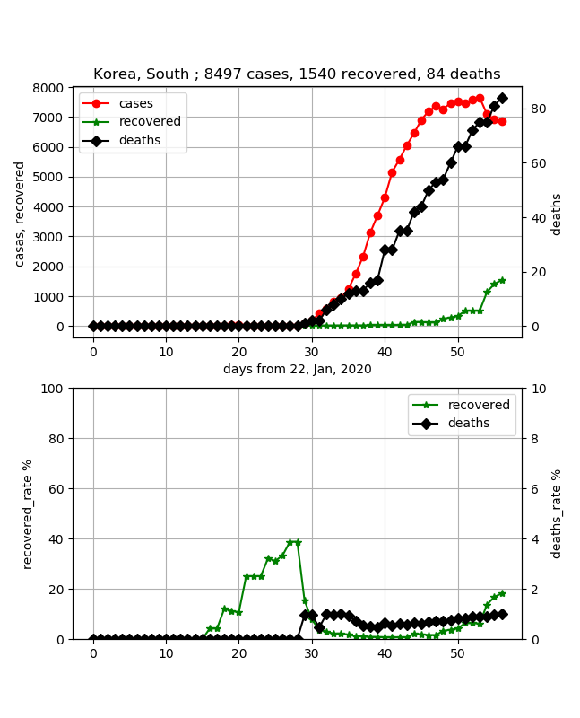 The mortality rate can be low. However, I heard that it has ended, and although the number of infections seems to have reached its peak, the cure rate is still less than 20%, and I have the impression that it is unpredictable. It simply takes about 30 days to reach 50%, and it seems that it will not go to the end until about 50 days after that.
- We are planning to make an app that can evaluate this a little more quantitatively.
·Italy
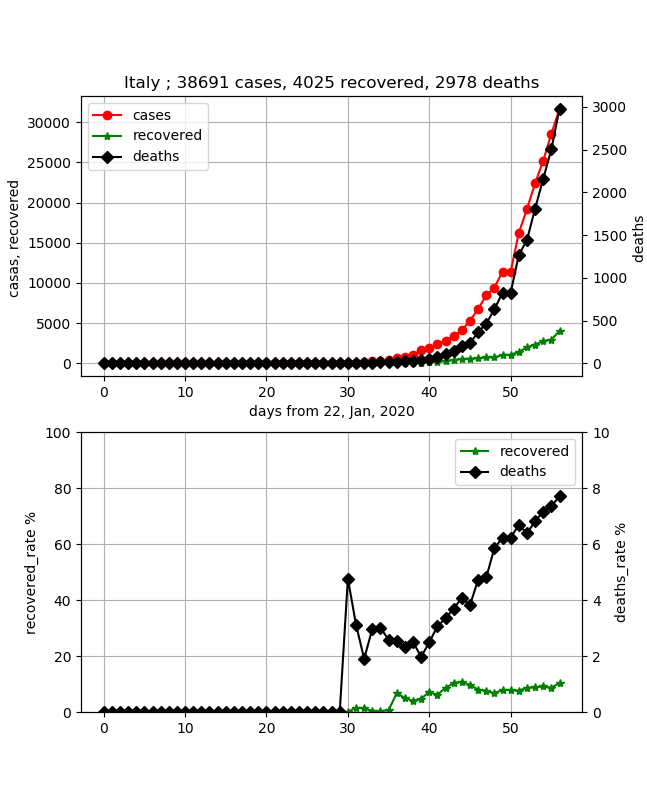 I was worried about the collapse of medical care, but I was relieved that the data was solid.
In other words, I feel that the country is in control. However, the characteristic is that the mortality rate is steadily rising and it is as high as about 8% recently. In addition, the cure rate is about 10%, and the number of infections is about 40,000, but it is in the midst of an increase, and there is no prospect of an end.
I was worried about the collapse of medical care, but I was relieved that the data was solid.
In other words, I feel that the country is in control. However, the characteristic is that the mortality rate is steadily rising and it is as high as about 8% recently. In addition, the cure rate is about 10%, and the number of infections is about 40,000, but it is in the midst of an increase, and there is no prospect of an end.
·Iran
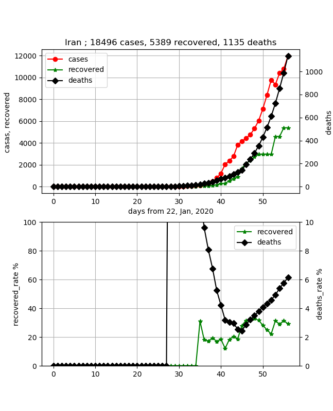 It is a worrying country along with Italy. After all, the mortality rate was an abnormal value, but when I came here, it increased sharply again and exceeded 6%. However, since the cure rate has reached about 30%, the number of infections may reach its peak soon. The increase in the cure rate is slow, but if the peak number of cures can be predicted from that, it is possible to reach containment.
Since the data has been solid, it seems that the collapse of medical care is okay.
It is a worrying country along with Italy. After all, the mortality rate was an abnormal value, but when I came here, it increased sharply again and exceeded 6%. However, since the cure rate has reached about 30%, the number of infections may reach its peak soon. The increase in the cure rate is slow, but if the peak number of cures can be predicted from that, it is possible to reach containment.
Since the data has been solid, it seems that the collapse of medical care is okay.
・ France / Germany / USA
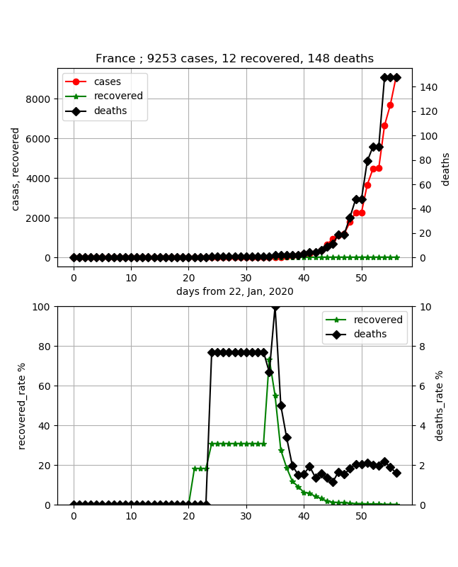
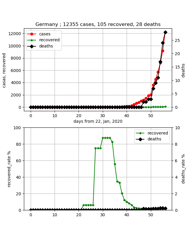 Shown together. Both countries are also worried. This is because the number of cases has increased in both cases, but the cure is almost zero. A sudden infection is predicted, and it can be imagined that this will not end for the time being.
The mortality rate is low at 2% in France, but it is almost 0 in Germany with less than 30 people. It's been less than 20 days since the infection, so I can imagine that many people are fighting illness, but I would like to see the transition.
The United States is also a country where the number of infections is increasing rapidly.
Shown together. Both countries are also worried. This is because the number of cases has increased in both cases, but the cure is almost zero. A sudden infection is predicted, and it can be imagined that this will not end for the time being.
The mortality rate is low at 2% in France, but it is almost 0 in Germany with less than 30 people. It's been less than 20 days since the infection, so I can imagine that many people are fighting illness, but I would like to see the transition.
The United States is also a country where the number of infections is increasing rapidly.
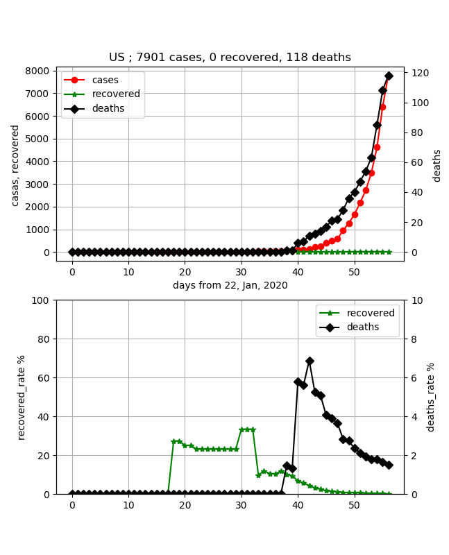 In the United States as well, the number of cures is 0 and the mortality rate is kept low at 2% or less, but this is also about 20 days after the rise of the number of infections, so I would like to see the transition.
·Spain
Spain is also one of the worried countries. It is as follows.
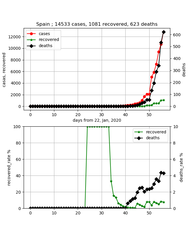 The data feels solid and controlled. However, the mortality rate is rising here as well, and has recently exceeded 4%. Looking at the cure rate, it is less than 10%, and the number of infections is about 15,000, but we can see that it is still in the early stages. I would like to keep an eye on future trends.
·Japan
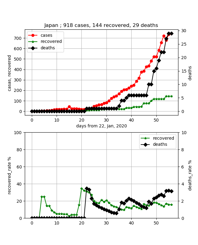 I think Japan is the country where the infection is spreading most slowly.
In a sense, I get the impression that it is both polar and Chinese.
The mortality rate was also kept low, but it seems that it is gradually approaching 4%. In addition, the cure rate has increased to about 18% now, but since it is increasing only very slowly, I think that neither the infection peak nor the cure rate peak can be seen yet. I think that it will be visible if it continues to increase for about 30 days. However, the increase in the number of infections is a downwardly convex curve, which may lead to a rapid increase, so I think it is unpredictable.
I think Japan is the country where the infection is spreading most slowly.
In a sense, I get the impression that it is both polar and Chinese.
The mortality rate was also kept low, but it seems that it is gradually approaching 4%. In addition, the cure rate has increased to about 18% now, but since it is increasing only very slowly, I think that neither the infection peak nor the cure rate peak can be seen yet. I think that it will be visible if it continues to increase for about 30 days. However, the increase in the number of infections is a downwardly convex curve, which may lead to a rapid increase, so I think it is unpredictable.
Summary
・ I tried plotting COVID-19 data ・ Multiple graphs could be associated and output ・ Evaluated what can be seen from the simulation with actual data
・ Extend the simulation so that the end can be predicted. ・ I want to make an app that categorizes the situation in each country.
Recommended Posts