[PYTHON] [Translation] scikit-learn 0.18 User Guide 2.8. Density estimation
Google translated http://scikit-learn.org/0.18/modules/density.html [scikit-learn 0.18 User Guide 2. Unsupervised Learning](http://qiita.com/nazoking@github/items/267f2371757516f8c168#2-%E6%95%99%E5%B8%AB%E3%81%AA From% E3% 81% 97% E5% AD% A6% E7% BF% 92)
2.8. Density estimation
Density estimation follows the line between unsupervised learning, feature engineering, and data modeling. Some of the most common and useful density estimation techniques are Gaussian Mixture ([sklearn.mixture.GaussianMixture](http://scikit-learn.org/0.18/modules/generated/sklearn.mixture.GaussianMixture.html#sklearn] Mixed models such as .mixture.GaussianMixture) and kernel density estimation (sklearn.neighbors.KernelDensity .neighbors.KernelDensity)) is a neighborhood-based approach. Gaussian mixing is described in more detail in the context of Clustering (http://scikit-learn.org/0.18/modules/clustering.html#clustering). It also serves as an unsupervised clustering scheme. Density estimation is a very simple concept, and most people are already familiar with the histogram, which is a common density estimation method.
2.8.1. Density estimation: Histogram
A histogram is a simple visualization of the data in which bins are defined, summarizing the number of data points in each bin. An example histogram is displayed in the upper left panel of the following figure.
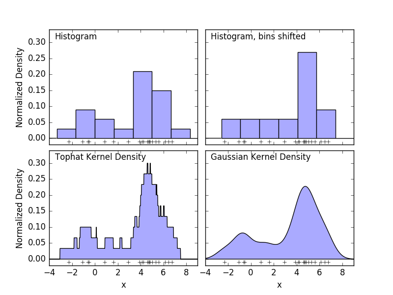
However, the big problem with histograms is that the choice of binning can have a disproportionate effect on the resulting visualization. Consider the upper right panel in the figure above. Shift the bin to the right to see a histogram of the same data. The results of the two visualizations may look quite different and the interpretation of the data may be different. Intuitively, you can think of the histogram as a stack of blocks, one block per point. Restore the histogram by stacking blocks in the appropriate grid space. But what if, instead of stacking blocks on a regular grid, we put each block in the center of the point it represents and sum the total height of each position? This idea leads to a visualization in the lower left. Perhaps not as clean as a histogram, but the fact that the data drives the position of the block means that it is a much better representation of the underlying data. This visualization is an example of kernel density estimation, in which case we use a top hat kernel (a square block of points). You can restore a smoother distribution by using a smoother kernel. The lower right plot shows the Gaussian kernel density estimate. Here, each point gives a Gaussian curve to the sum. The result is a smooth density estimate derived from the data, which acts as a powerful nonparametric model of the point distribution.
2.8.2. Kernel density estimation
Kernel density estimation in scikit-learn is sklearn.neighbors.KernelDensity As an estimator It is implemented. It uses a ball tree or k-d tree for efficient queries (see Nearest Neighbors for these discussions). please refer to). The above example uses a 1D dataset for simplicity, but kernel density estimation can be performed in any number of dimensions. However, in reality, the dimensional curse reduces performance at a higher level.
The following figure draws 100 points from the bimodal distribution and provides kernel density estimates for the three kernel choices.
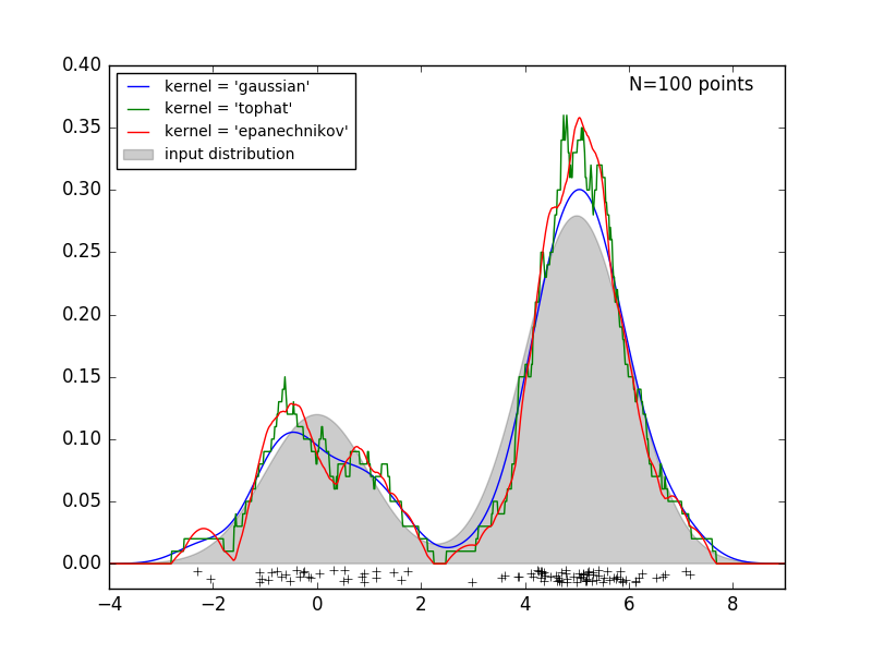
It is clear how the kernel shape affects the smoothness of the resulting distribution. The scikit-learn kernel density estimator can be used as follows:
>>> from sklearn.neighbors.kde import KernelDensity
>>> import numpy as np
>>> X = np.array([[-1, -1], [-2, -1], [-3, -2], [1, 1], [2, 1], [3, 2]])
>>> kde = KernelDensity(kernel='gaussian', bandwidth=0.2).fit(X)
>>> kde.score_samples(X)
array([-0.41075698, -0.41075698, -0.41076071, -0.41075698, -0.41075698,
       -0.41076071])
Here we are using kernel ='gaussian' as above. Mathematically, the kernel is a positive function $ K (x; h) $, which is controlled by the bandwidth parameter $ h $. Given this kernel format, the density estimate at point y in point cloud N is given by:
\rho_K(y) = \sum_{i=1}^{N} K((y - x_i) / h)
Bandwidth here acts as a smoothing parameter and controls the trade-off between bias and variance in the results. Wide bandwidth results in a very smooth (ie, high bias) density distribution. Narrow bandwidth results in a non-smooth (ie, highly dispersed) density distribution.
sklearn.neighbors.KernelDensity implements some common kernel formats. This is shown in the following figure.
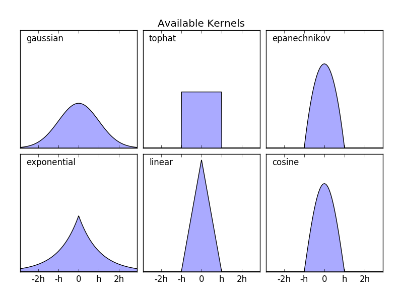
The format of these kernels is:
- Gaussian kernel
kernel ='gaussian'K(x; h) \propto \exp(- \frac{x^2}{2h^2} )
- Tophat kernel
kernel ='tophat'K(x; h) \propto 1 if x < h
- Epanechnikov kernel
kernel ='epanechnikov'K(x; h) \propto 1 - \frac{x^2}{h^2}
- Exponential kernel
kernel ='exponential'K(x; h) \propto \exp(-x/h)
- Linear kernel
kernel ='linear'K(x; h) \propto 1 - x/h if x < h
- Cosine kernel
kernel ='cosine'K(x; h) \propto \cos(\frac{\pi x}{2h}) if x < h
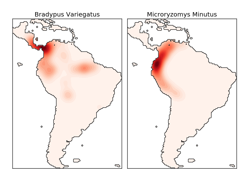
The kernel density estimate uses a valid distance metric (sklearn.neighbors.DistanceMetric). You can use any of them (see), but the results are properly normalized only for Euclidean metrics. One particularly useful metric is the Haversine Distance (https://en.wikipedia.org/wiki/Haversine_formula), which measures the angular distance between points on a sphere. The following example uses kernel density estimation for visualization of geospatial data. In this example, it is the distribution of observations of two different species in South America:
Another useful application of kernel density estimation is to train a nonparametric generative model of a dataset in order to efficiently derive new samples from this generative model. Here is an example of using this process to create a new set of handwritten digits using the Gaussian kernel learned in PCA projection of data.
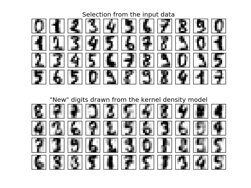
The "new" data consists of a linear combination of the input data and is stochastically drawn assuming a KDE model.
- Example:
- Simple 1D kernel density estimation: 1 Calculation of simple kernel density estimates in dimensions.
- Kernel density estimation: Card density An example of using estimation to train a generative model of handwritten numeric data and draw a new sample from this model.
- Kernel density estimation of species distribution: Geography An example of kernel density estimation using Haversine distance metric for visualizing spatial data
[scikit-learn 0.18 User Guide 2. Unsupervised Learning](http://qiita.com/nazoking@github/items/267f2371757516f8c168#2-%E6%95%99%E5%B8%AB%E3%81%AA From% E3% 81% 97% E5% AD% A6% E7% BF% 92)
© 2010 --2016, scikit-learn developers (BSD license).