[PYTHON] [Translation] scikit-learn 0.18 User Guide 2.5. Decompose the signal in the component (matrix factorization problem)
Google translated http://scikit-learn.org/0.18/modules/decomposition.html
[User Guide Table of Contents](http://qiita.com/nazoking@github/items/267f2371757516f8c168#2-%E6%95%99%E5%B8%AB%E3%81%AA%E3%81%97%E5 % AD% A6% E7% BF% 92)
2.5. Decompose the signal in the component (matrix factorization problem)
2.5.1. Principal component analysis (PCA)
2.5.1.1. Accurate PCA and probabilistic interpretation
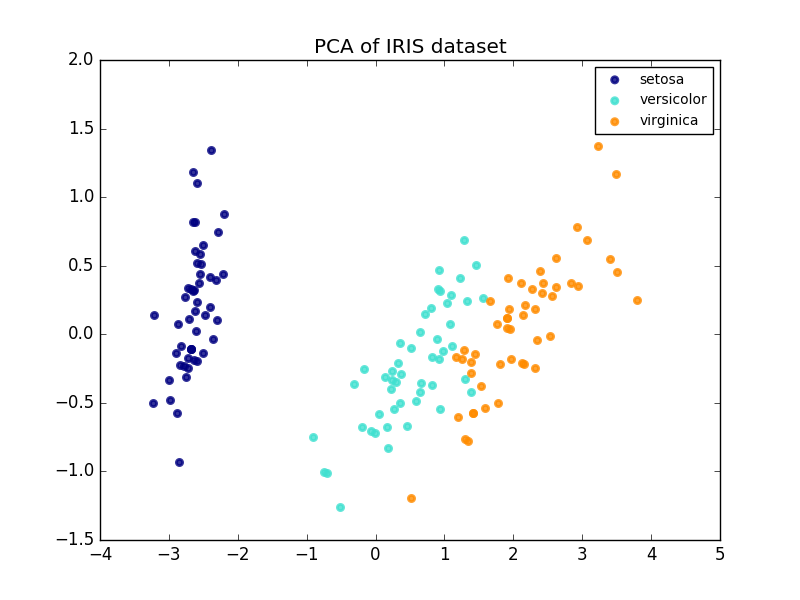
PCA is used to decompose multivariate datasets in a set of consecutive orthogonal components that explain the maximum amount of variance. In scikit-learn, PCA uses the fit method for n components. It is implemented as a transformer object that trains and projects to these components with new data.
The optional parameter whiten = True allows you to project data into a singular space while scaling each component to unit variance. This is often useful if the downstream of the model strongly presupposes signal isotropic. This is the case, for example, with a support vector machine using the RBF kernel and the K-Means clustering algorithm.
The following is an example of an Iris dataset. It consists of four features, projected onto two dimensions, and describes most variances.
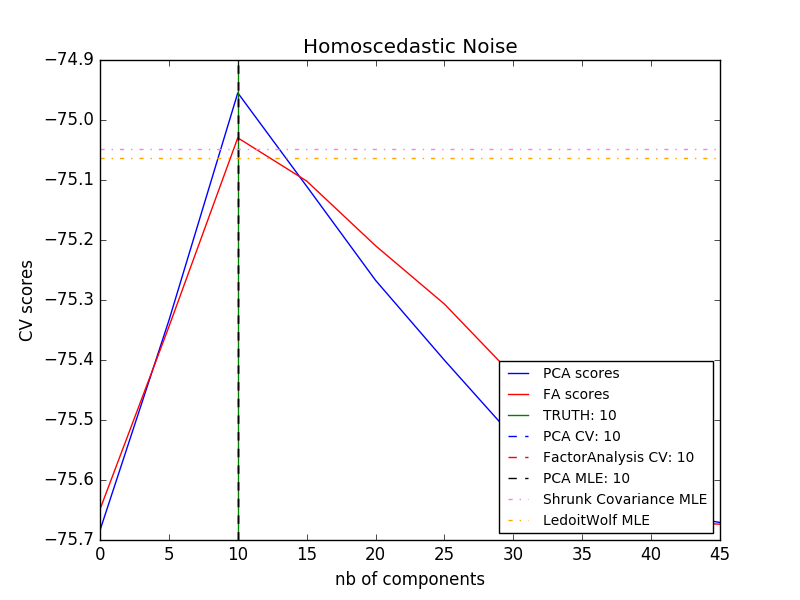
The PCA object also provides a stochastic interpretation of the PCA, which can give data potential based on the variance it describes. In this way, we implement a score method that can be used for mutual authentication.
- Example:
- [Comparison of LDA and PCA 2D projections of Iris dataset](http://scikit-learn.org/0.18/auto_examples/decomposition/plot_pca_vs_lda.html#sphx-glr-auto-examples-decomposition-plot-pca-vs -lda-py)
- [Model selection by probabilistic PCA and factor analysis (FA)](http://scikit-learn.org/0.18/auto_examples/decomposition/plot_pca_vs_fa_model_selection.html#sphx-glr-auto-examples-decomposition-plot-pca- vs-fa-model-selection-py)
2.5.1.2. Incremental PCA
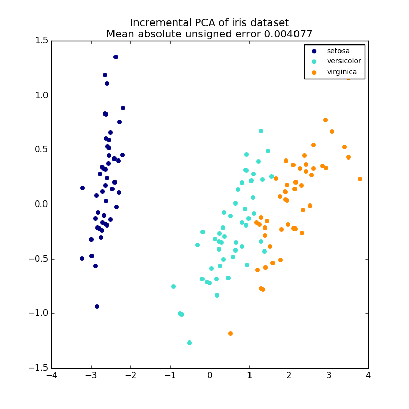
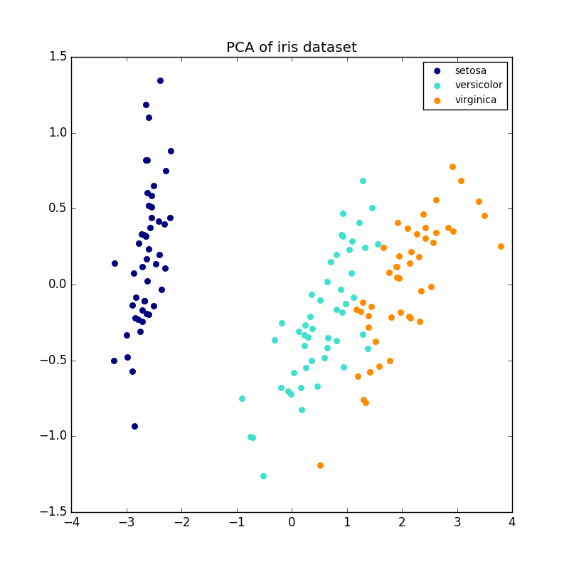
PCA Objects are very useful, but have certain limitations for large datasets. there is. PCA only supports batch processing, so all the data processed must fit in main memory. IncrementalPCA Objects use a different form of processing and are similar to the results of PCA. It allows for partial calculations that match exactly and processes the data in a mini-batch way. IncrementalPCA allows you to implement off-core principal component analysis in any of the following ways:
- Use the
partial_fitmethod for chunks of data fetched sequentially from your local hard drive or network database. - Call the
fitmethod on a memory-mapped file usingnumpy.memmap.
IncrementalPCA only stores component and noise variance estimates and updates ʻexplain_variance_ratio_` in stages. For this reason, memory usage depends on the number of samples per batch, not the number of samples processed by the dataset.
- Example:
- Incremental PCA
2.5.1.3. PCA with Random SVD
It is often interesting to project data into a low-dimensional space that preserves most variances by removing the component's singular vectors associated with more singular values.
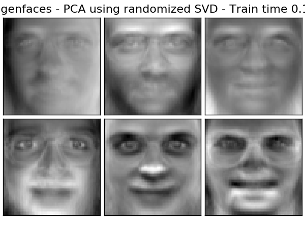
For example, when dealing with a 64x64 pixel gray level image for face recognition, the data dimension is 4096, and training an RBF support vector machine for such a wide range of data is slow. In addition, all images of the human face are somewhat similar, so we can see that the intrinsic dimension of the data is much less than 4096. The sample is on a manifold of a much lower dimension (eg, about 200). The PCA algorithm can be used to linearly transform the data, while at the same time reducing the dimensions and preserving most of the variance described.
The PCA class used in the optional parameter svd_solver ='randomized' is very useful in such cases. It is much more efficient to limit the calculation to approximate estimates of the singular vector, as it removes most singular vectors. Please actually perform the conversion.
For example, here are 16 sample portraits (centered around 0.0) from the Olivetti dataset. On the right is the first 16 singular vectors reconstructed as portraits. The calculation time is less than 1 second because only the top 16 singular vectors of the dataset of $ n_ {samples} = 400 $ and $ n_ {features} = 64 \ times 64 = 4096 $ are required.
Note: You must also use the optional parameter svd_solver ='randomized' to give the PCA the size of the low-dimensional space n_components as a required input parameter.
Focusing on $ n_ {max} = max (n_ {samples}, n_ {features}) $ and $ n_ {min} = min (n_ {samples}, n_ {features}) $, the time complexity of randomized PCA Is $ O (n_ {max} ^ 2 \ cdot n_ {min}) $ instead of $ O (n_ {max} ^ 2 \ cdot n_ {components}) $ in the exact method implemented in PCA.
Randomized PCA memory footprint is $ n_ {max} in the exact way
It is proportional to $ 2 \ cdot n_ {max} \ cdot n_ {components} $ instead of \ cdot n_ {min} $.
Note: The implementation of ʻinverse_transform in PCA with svd_solver ='randomized'is not the exact inverse transform oftransform even with whiten = False` (default).
- Example:
- Example of recognition using eigenface and SVM
- Face Dataset Decomposition (http://scikit-learn.org/0.18/auto_examples/decomposition/plot_faces_decomposition.html#sphx-glr-auto-examples-decomposition-plot-faces-decomposition-py)
- References:
- Find a structure with randomness: a probabilistic algorithm for constructing an approximate matrix factorization Halko, et al. , 2009
2.5.1.4. Kernel PCA
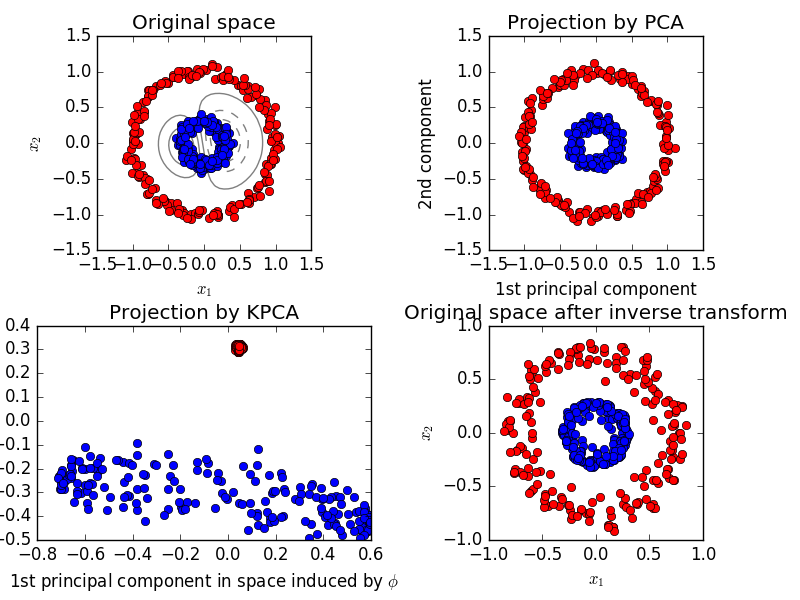
KernelPCA is an extension of PCA that realizes nonlinear dimensionality reduction by using the kernel. (See Pair Metrics, Affinity and Kernel (http://scikit-learn.org/0.18/modules/metrics.html#metrics)). It has many applications such as denoising, compression, and structured prediction (kernel dependency estimation). KernelPCA supports both transform and ʻinverse_transform`.
- Example:
- Kernel PCA
2.5.1.5. Sparse Principal Component Analysis (SparsePCA and MiniBatchSparsePCA)
SparsePCA extracts the set of sparse components that best reconstruct data. It is a variant of PCA for the purpose of doing so. MiniBatchSparsePCA (MiniBatchSparsePCA) is a variant of SparsePCA and is faster. However, the accuracy is inferior. The increased speed is achieved by repeating small chunks of the feature set for a specified number of iterations. Principal component analysis (PCA) has the disadvantage that the components extracted by this method have an exclusively dense representation, i.e. a non-zero coefficient when expressed as a linear combination of the original variables. This can be difficult to interpret. In many cases, the actual underlying component can be more naturally imagined as a sparse vector. For example, in face recognition, components may naturally map to parts of the face. The sparse principal component clearly emphasizes which of the original features contributes to the differences between the samples, resulting in a more concise and interpretable representation. The following example shows 16 components extracted using SparsePCA from a dataset on the Olivetti face. You can see how the normalization term derives many zeros. Moreover, the natural structure of the data makes the nonzero coefficients vertically adjacent. The model does not force this mathematically. Each component is a vector $ h \ in \ mathbf {R} ^ {4096} $, and there is no concept of vertical adjacency except during human-friendly visualizations such as 64 x 64 pixel images. The fact that the components shown below appear locally is an effect of the unique structure of the data, and such local patterns minimize reconstruction error. There are norms that induce sparseness considering adjacency and various types of structures. See [Jen09] for a review of such methods. For more information on using sparse PCA, see the example section below.
Note that there are many different expressions in the SparsePCA problem. What is implemented here is based on [Mrl09]. The resolved optimization problem is the PCA problem (dictionary learning), which has a $ \ ell_1 $ penalty on the component.
(U^*, V^*) = \underset{U, V}{\operatorname{arg\,min\,}} & \frac{1}{2}
             ||X-UV||_2^2+\alpha||V||_1 \\
             \text{subject to\,} & ||U_k||_2 = 1 \text{ for all }
             0 \leq k < n_{components}
The $ \ ell_1 $ norm, which induces sparsity, also protects the learning component from noise when few training samples are available. The degree of penalty (and therefore sparsity) can be adjusted via the hyperparameter ʻalpha`. Small values result in a loosely regularized factorization, and large values reduce many coefficients to zero.
** Note: ** In the online algorithm, the MiniBatchSparsePCA class is partial_fit. It doesn't implement because the algorithm is online along the feature direction, not the sample direction.
- Example:
- Decompose face dataset (http://scikit-learn.org/0.18/auto_examples/decomposition/plot_faces_decomposition.html#sphx-glr-auto-examples-decomposition-plot-faces-decomposition-py)
- References:
- \ [Mrl09] Learning an online dictionary for sparse coding J. Mairal, F. Bach, J. Ponce, G. Sapiro, 2009
- \ [Jen09] Structured Sparse PCA Analysis R. Jenatton, G. Obozinski , F. Bach, 2009
2.5.2. Truncated singular value decomposition and latent semantic analysis
In TruncatedSVD, $ k $ is a user-specified parameter. Implements a variant of Singular Value Decomposition (SVD) that calculates only the maximum singular value of.
When the truncated SVD is applied to a term-document matrix (returned by CountVectorizer or TfidfVectorizer), this transformation is done in latent semantic analysis (LSA). Known as .edu / IR-book / pdf / 18lsi.pdf). This is to transform the matrix into a lower dimensional "semantic" space. In particular, LSAs are known to combat the effects of synonyms and polysemous words (both roughly meaning multiple meanings). This indicates that the term document matrix is overly sparse and has low similarity by means such as cosine similarity.
** Note: ** LSA, also known as latent indexing, LSI, is strictly used for persistent indexes for information retrieval purposes.
Mathematically, the truncated SVD applied to the training sample $ X $ produces a low-rank approximation $ X $.
X \approx X_k = U_k \Sigma_k V_k^\top
After this operation, $ U_k \ Sigma_k ^ \ top $ is a transformed training set with $ k $ features (called n_components in the API).
It also multiplies $ V_k $ to convert the test set $ X $.
X' = X V_k
** Note: ** Most processing of LSAs in the Natural Language Processing (NLP) and Information Retrieval (IR) literature swaps the axes of the matrix $ n $ so that they have the form n_features x n_samples. I will. We present LSAs in different ways that match the scikit-learn API well, but the singular values found are the same.
TruncatedSVD is very similar to PCA, except that it works directly on the sample matrix $ X $ instead of the covariance matrix. Subtracting the average of $ X $ in the column direction (per feature) from the feature, the resulting truncated matrix SVD is equivalent to PCA. In practice, this does not densify the scipy.sparse matrix because the Truncated SVD converter can fill up memory even with medium density document collections. Means to accept.
The TruncatedSVD transducer works with any (sparse) feature matrix, but its use with the tf-idf matrix is recommended over the unprocessed frequency count in the LSA / document processing settings. In particular, to make up for LSA's false assumptions about textual data, sublinear scaling and inverse document frequency should be turned on to bring feature values closer to a Gaussian distribution (sublinear_tf = True, ʻuse_idf =". True`).
- Example:
- Clustering text documents using k-means
- References:
- Christopher D. Manning, Prabhakar Raghavan and Hinrich Schütze (2008), Cambridge University Press, Chapter 18: Matrix Decomposition and Potential Indexing .pdf)
2.5.3. Dictionary learning
2.5.3.1. Sparse coding with pre-computed dictionaries
SparseCoder The object is a fixed precomputed signal, such as a discrete wavelet base. An estimator that can be used to convert to a sparse linear combination from a dictionary. Therefore, this object does not implement the fit method. This conversion becomes a sparse coding problem. Finding a representation of the data as a linear combination of as few dictionary atoms as possible. All variations of dictionary learning implement the following transformation methods that can be controlled via the transform_method initialization parameters.
- Pursuit of Orthogonal Matching (OMP: Orthogonal Matching Pursuit)
- Minimum angle regression (Minimum angle regression)
- Lasso calculated by minimum angle regression
- Lasso using coordinate descent (Lasso)
- Threshold
The thresholds are very fast, but they cannot be reconstructed accurately. They have been shown to be useful in the literature for classification work. For image reconstruction tasks, orthogonal matching tracking provides the most accurate and unbiased reconstruction.
The dictionary learning object provides the possibility of separating positive and negative values in the result of sparse coding via the split_code parameter. This is dictionary learning to extract features used in supervised learning so that the learning algorithm can assign different weights from positive to negative loads corresponding to the negative load of a particular atom. This is useful when using.
The split code for one sample has a length of 2 * n_components and is created using the following rules: First, the usual code of length n_components is calculated. The first n_components entry for split_code is then filled with the positive part of the regular code vector. The second half of the split code is filled with the negative part of the code vector with only positive signs. Therefore, split_code is not negative.
2.5.3.2. General dictionary learning
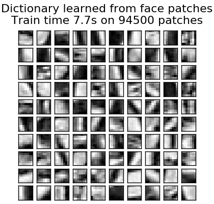
Dictionary learning (DictionaryLearning) is to sparsely encode matching data. It is a matrix factorization problem that corresponds to finding a (usually excessive) dictionary that works well with. Representing the data as a dilute combination of atoms from the overcomplete dictionary suggests the work of the major mammalian visual cortex. As a result, dictionary learning applied to image patches has been shown to give good results in image processing tasks such as image completion, repair and denoising, and monitored recognition tasks. Dictionary learning is an optimization problem that is solved by updating the sparse code as an alternative and modifying the dictionary to best fit the sparse code as a solution to multiple lasso problems. ..
(U^*, V^*) = \underset{U, V}{\operatorname{arg\,min\,}} & \frac{1}{2}
             ||X-UV||_2^2+\alpha||U||_1 \\
             \text{subject to\,} & ||V_k||_2 = 1 \text{ for all }
             0 \leq k < n_{atoms}
After adapting to a dictionary using these steps, transformation is a simple coding step that shares the same implementation with all dictionary learning objects ([Sparse coding with pre-calculated dictionaries](http: //) See scikit-learn.org/0.18/modules/decomposition.html#sparsecoder). The following image shows how the dictionary was learned from a 4x4 pixel image patch extracted from a portion of the raccoon's face image.
- Example:
- Image noise reduction using dictionary learning
- References:
- "Learning Online Dictionaries for Sparse Coding" J. Mairal, F. Bach, J. Ponce, G. Sapiro, 2009
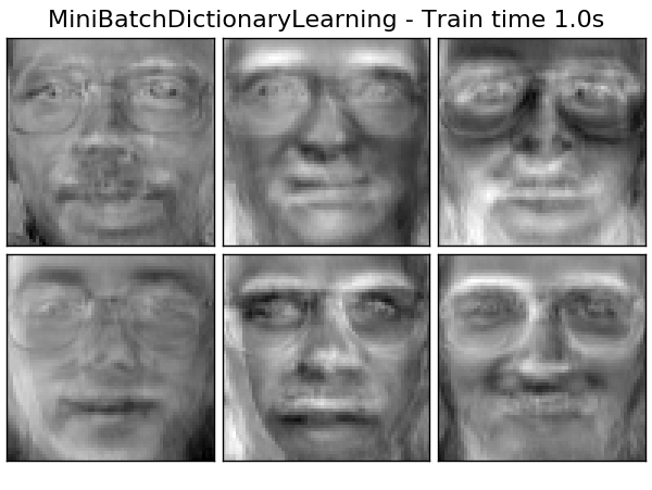
2.5.3.3. Mini-batch dictionary learning
MiniBatchDictionaryLearning (http://scikit-learn.org/0.18/modules/generated/sklearn.decomposition.MiniBatchDictionaryLearning.html#sklearn.decomposition.MiniBatchDictionaryLearning) is a faster dictionary learning algorithm for large datasets. However, it implements a less accurate version.
By default, MiniBatchDictionaryLearning divides the data into mini-batch and optimizes it online by circulating the mini-batch a specified number of iterations. However, it does not implement a stopped state at this time.
The estimator also implements partial_fit. This will update the dictionary only once in a mini-batch. It can be used for online learning when the data is not readily available from the beginning or when the data does not fit in memory.
** Clustering for dictionary learning **
Note that clustering can be a good proxy for learning a dictionary when using dictionary learning to extract expressions (eg in the case of sparse coding). For example, the MiniBatchKMeans estimator is computationally efficient and the partial_fit method. Conduct online learning using.
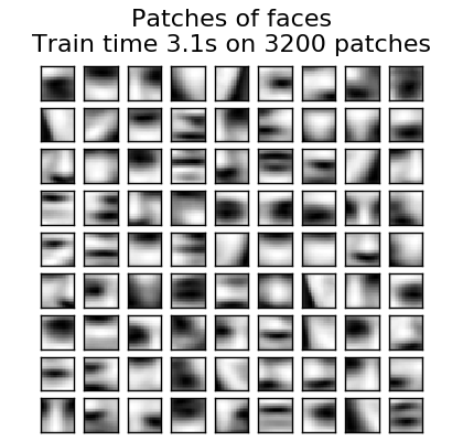
- Example: [Online learning of face parts dictionary](http://scikit-learn.org/0.18/auto_examples/cluster/plot_dict_face_patches.html#sphx-glr-auto-examples-cluster-plot-dict-face-patches -py)
2.5.4. Factor analysis
In unsupervised learning, the dataset is $ X = \ {x_1, x_2, \ dots, x_n There is only } $. How can this dataset be described mathematically? In a very simple continuous latent variable model, $ X $ is
x_i = W h_i + \mu + \epsilon
The vector $ h \ _i $ is not observed and is therefore called "latent". $ ε $ is considered a noise term distributed according to a Gaussian distribution with mean 0 and covariance $ \ Psi $ (ie $ \ epsilon \ sim \ mathcal {N} (0, \ Psi)) $). $ Μ $ is any offset vector. Such a model is called "generative" because it describes how $ x \ _i $ is generated from $ h \ _i $. Using all $ x \ _i $ as columns to create the matrix $ \ mathbf {X} $ and all $ h_i $ as columns in the matrix $ \ mathbf {H} $ (well defined) You can write (using $ \ mathbf {M} $ and $ \ mathbf {E} $) as follows:
\mathbf{X} = W \mathbf{H} + \mathbf{M} + \mathbf{E}
In other words, we decomposed the matrix $ \ mathbf {X} $. Given $ h_i $, the above equation automatically means the following stochastic interpretation.
p(x_i|h_i) = \mathcal{N}(Wh_i + \mu, \Psi)
For the perfect probability model, we also need a prior distribution for the latent variable $ h $. The simplest assumption based on the good characteristics of the Gaussian distribution is $ h \ sim \ mathcal {N} (0, \ mathbf {I}) $. This produces a Gaussian distribution as the marginal distribution of $ x $:
p(x) = \mathcal{N}(\mu, WW^T + \Psi)
Now, without further assumptions, the idea of having a latent variable $ h $ would be superfluous. $ x $ can be fully modeled with mean and covariance. We need to impose a more specific structure on one of these two parameters. A simple additional assumption is about the structure of the error covariance $ \ Psi $:
- $ \ Psi = \ sigma ^ 2 \ mathbf {I} $: This assumption leads to a probabilistic model of PCA.
- $ \ Psi = diag (\ psi_1, \ psi_2, \ dots, \ psi_n) $: This model is a classic statistical model Factor Analysis [http://scikit-learn.org/0.18/modules] It is called /generated/sklearn.decomposition.FactorAnalysis.html#sklearn.decomposition.FactorAnalysis). The matrix W is sometimes referred to as the "factor loading matrix".
Both models essentially estimate a Gaussian distribution with a low-ranked covariance matrix. Both models are stochastic and can be integrated into more complex models. For example, a combination of factor analyzes. Very different models (eg FastICA when non-Gaussian prior probabilities on latent variables are assumed. .decomposition.FastICA)) is obtained. Factor analysis translates similar components (columns of its loading matrix) into PCA Can be generated. However, it is not possible to make a general description of these components (eg, whether they are orthogonal).
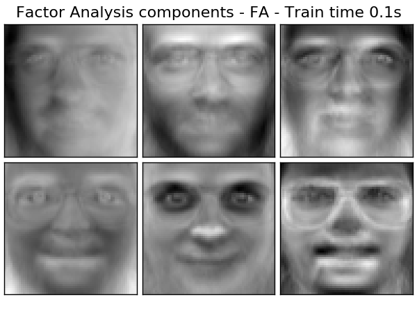
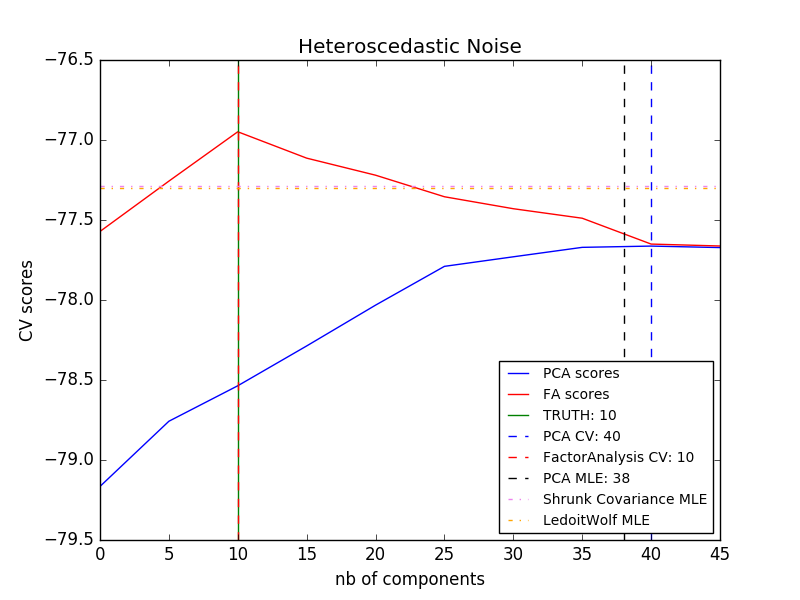
The main advantage of factor analysis over PCA is in all directions of the input space. The ability to model the variances individually (heteroscedastic noise).
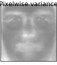
This allows better model selection than stochastic PCA in the presence of anisotropic noise.
- Example:
- [Model selection by probabilistic PCA and factor analysis (FA)](http://scikit-learn.org/0.18/auto_examples/decomposition/plot_pca_vs_fa_model_selection.html#sphx-glr-auto-examples-decomposition-plot-pca- vs-fa-model-selection-py)
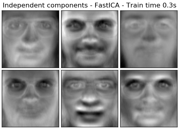
2.5.5. Independent Component Analysis (ICA)
Independent component analysis separates multivariate signals into maximally independent additive subcomponents. FastICA Implemented in scikit-learn using the algorithm. Typically, ICA is used to separate superimposed signals, not to reduce dimensionality. The ICA model does not contain a noise term, so whitening must be applied for the model to be correct. This can be done internally using the whiten argument or manually using PCA or one of its variants. It is classically used to separate mixed signals, as in the example below (a problem called blind separation).
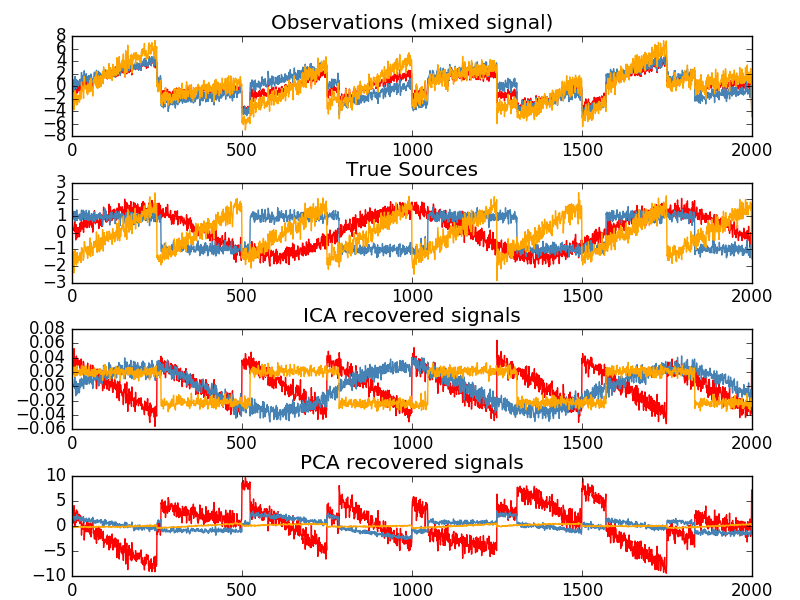
The ICA can also be used as yet another non-linear decomposition that finds sparse components.
- Example:
- [Separation of blind sources using FastICA](http://scikit-learn.org/0.18/auto_examples/decomposition/plot_ica_blind_source_separation.html#sphx-glr-auto-examples-decomposition-plot-ica-blind-source- separation-py)
- 2D Point Cloud FastICA
- Face Dataset Decomposition (http://scikit-learn.org/0.18/auto_examples/decomposition/plot_faces_decomposition.html#sphx-glr-auto-examples-decomposition-plot-faces-decomposition-py)
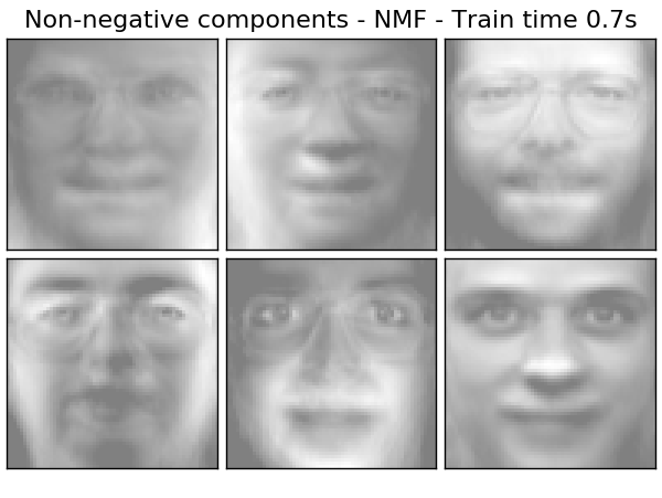
2.5.6. Non-negative matrix factorization (NMF or NNMF)
2.5.6.1. NMF with Frobenius norm
NMF is a decomposition that assumes that the data and components are non-negative. This is an alternative approach. If the data matrix does not contain negative values, you can insert NMF instead of PCA or its variants. By optimizing the distance $ d $ between $ X $ and the matrix product $ WH $, we find the decomposition of the sample $ X $ into two matrices $ W $ and $ H $. The most widely used distance function is the squared Frobenius norm, which is an obvious extension to the Euclidean distance matrix.
d_{\mathrm{Fro}}(X, Y) = \frac{1}{2} ||X - Y||_{\mathrm{Fro}}^2 = \frac{1}{2} \sum_{i,j} (X_{ij} - {Y}_{ij})^2
Unlike PCA, the representation of a vector is obtained additively by superimposing the components without subtraction. Such an additive model is useful for representing images and text.
In [Hoyer, 04], it is observed that NMF produces a parts-based representation of a dataset and becomes an interpretable model when carefully constrained. The following example shows 16 dilute components found by NMA in comparison to a PCA-specific surface from an image of the Olivetti face dataset.
 The ʻinit
attribute determines which initialization method is applied. This has a significant impact on method performance. NMF implements the non-negative double singular value decomposition method (NNDSVD). NNDSVD is based on two SVD processes that approximate the data matrix, and the other approximating positive sections of the resulting partial SVD coefficients take advantage of the algebraic properties of the unit rank matrix. The basic NNDSVD algorithm is suitable for sparse factorization. For high densities, its variants NNDSVDa (all zeros are set equal to the average of all elements of the data) and NNDSVDar (where zero is a random perturbation smaller than the average of the data divided by 100). Is set to) is recommended. NMF can also be initialized with a properly scaled random non-negative matrix by setting ʻinit = "random". You can also pass an integer seed or RandomState to random_state to control reproducibility.
NMF allows you to add L1 and L2 functions to the loss function to normalize the model. L2 prior uses the Frobenius norm and L1 prior uses the element unit L1 norm. Like ElasticNet, the combination of L1 and L2 is controlled by the l1_ratio ($ \ rho
\alpha \rho ||W||_1 + \alpha \rho ||H||_1
+ \frac{\alpha(1-\rho)}{2} ||W||_{Fro} ^ 2
+ \frac{\alpha(1-\rho)}{2} ||H||_{Fro} ^ 2
The normalized objective function is:
\frac{1}{2}||X - WH||_{Fro}^2
+ \alpha \rho ||W||_1 + \alpha \rho ||H||_1
+ \frac{\alpha(1-\rho)}{2} ||W||_{Fro} ^ 2
+ \frac{\alpha(1-\rho)}{2} ||H||_{Fro} ^ 2
NMF normalizes both W and H. The function non_negative_factorization has finer control over normalization attributes and can normalize W, H only, or both.
- Example:
- Face Dataset Decomposition (http://scikit-learn.org/0.18/auto_examples/decomposition/plot_faces_decomposition.html#sphx-glr-auto-examples-decomposition-plot-faces-decomposition-py)
- [Topic Extraction Using Non-Negative Matrix Factorization and Latent Dirichlet Allocation](http://scikit-learn.org/0.18/auto_examples/applications/topics_extraction_with_nmf_lda.html#sphx-glr-auto-examples-applications-topics- extraction-with-nmf-lda-py)
- References:
- "Learning of object parts by non-negative matrix factorization" D. Lee, S. Seung, 1999
- "Factorization of nonnegative matrices with sparseness constraints" P. Hoyer, 2004
- "Projection Gradient Method for Non-Negative Matrix Factorization" C.-J. Lin, 2007
- "SVD-based initialization: beginning of nonnegative matrix factorization" C. Boutsidis, E. Gallopoulos, 2008
- "Fast local algorithm for large-scale nonnegative matrix and tensor decomposition" A. Cichocki, P. Anh-Huy, 2009
2.5.7. Latent Dirichlet Allocation (LDA)
The Latent Dirichlet Allocation is a generative probabilistic model for collecting discrete datasets such as text corpora. It is also the topic model used to discover abstract topics from a collection of documents. The LDA graphical model is a 3-level Bayesian model.
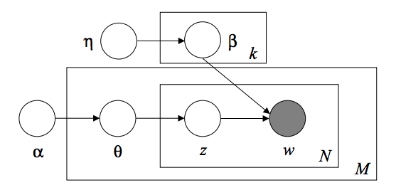
When modeling a text corpus, the model assumes the following generation process for a corpus with D documents and K topics.
- For each topic $ k $, $ \ beta_k \ sim Dirichlet (\ eta), : k = 1 ... K $
- For each document $ d $, $ \ theta_d \ sim Dirichlet (\ alpha), : d = 1 ... D $
- For each word $ i $ in the document $ d $:
- Draw topic index $ z_ {di} \ sim Multinomial (\ theta_d) $
- Depict the observed word $ w_ {ij} \ sim Multinomial (beta_ {z_ {di}}.) $
For parameter estimation, the posterior distribution is:
p(z, \theta, \beta |w, \alpha, \eta) =
  \frac{p(z, \theta, \beta|\alpha, \eta)}{p(w|\alpha, \eta)}
Since the backwards are awkward, the variational Bayesian method uses a simpler distribution to approximate $ q (z, \ theta, \ beta | \ lambda, \ phi, \ gamma) $ and their variational parameters $ . lambda, \ phi, \ gamma $ are optimized to maximize Evidence Lower Bound (ELBO).
log\: P(w | \alpha, \eta) \geq L(w,\phi,\gamma,\lambda) \overset{\triangle}{=}
  E_{q}[log\:p(w,z,\theta,\beta|\alpha,\eta)] - E_{q}[log\:q(z, \theta, \beta)]
Maximizing the ELBO is a Kullback-Leibler between $ q (z, \ theta, \ beta) $ and the true posterior $ p (z, \ theta, \ beta | w, \ alpha, \ eta) $. Equivalent to minimizing the difference in (KL).
LatentDirichletAllocation implements the online variational Bayesian algorithm for online and batch updates. Supports both methods. The batch method updates the variable variable after passing each full path to the data, while the online method updates the variable variable from the mini-batch data point.
** Note: ** The online method is guaranteed to converge to the local optimum point, but the quality and convergence speed of the optimum point may depend on the mini-batch size and attributes associated with the learning speed setting.
When LatentDirichletAllocation is applied to the "Document-Terms" matrix, the matrix is decomposed into a "Topic-Terms" matrix and a "Document-Topics" matrix. The "topic-terms" matrix is stored in the model as components_, but you can calculate the" document-topic "matrix with the transform method.
LatentDirichletAllocation also implements the partial_fit method. This is used when data is retrieved continuously.
- Example:
- [Topic Extraction Using Non-Negative Matrix Factorization and Latent Dirichlet Allocation](http://scikit-learn.org/0.18/auto_examples/applications/topics_extraction_with_nmf_lda.html#sphx-glr-auto-examples-applications-topics- extraction-with-nmf-lda-py)
- References:
- Latent Dirichlet Allocation D. Bray, A. N, M. Jordan, 2003
- Online Learning for Latent Dirichlet Allocation M. Hoffman, D.Blei, F.Bach, 2010
- Stochastic variational reasoning M. Hoffman, D.Blei, C.Wang, J.Pasley, 2013
[User Guide Table of Contents](http://qiita.com/nazoking@github/items/267f2371757516f8c168#2-%E6%95%99%E5%B8%AB%E3%81%AA%E3%81%97%E5 % AD% A6% E7% BF% 92)
© 2010 --2016, scikit-learn developers (BSD license).