Google translated http://scikit-learn.org/0.18/modules/calibration.html [scikit-learn 0.18 User Guide 1. Supervised Learning](http://qiita.com/nazoking@github/items/267f2371757516f8c168#1-%E6%95%99%E5%B8%AB%E4%BB%98 From% E3% 81% 8D% E5% AD% A6% E7% BF% 92)

1.16. Probability calibration

When performing a classification, we often not only predict the class labels, but also get the probabilities of each label. This probability gives some confidence in the prediction. Some models have poor estimates of class probabilities, while others do not support probability prediction. Calibration modules allow you to better adjust the probabilities of a particular model or add support for probabilistic prediction. A well-calibrated classifier is a stochastic classifier that can directly interpret the output of the predict_proba method as a confidence level. For example, about 80% of samples given a predict_proba value of 0.8 by a well-calibrated (binary) classifier actually belong to the positive class. The following plot compares how well the stochastic predictions of the various classifiers are calibrated.

較正プロット（信頼性曲線）

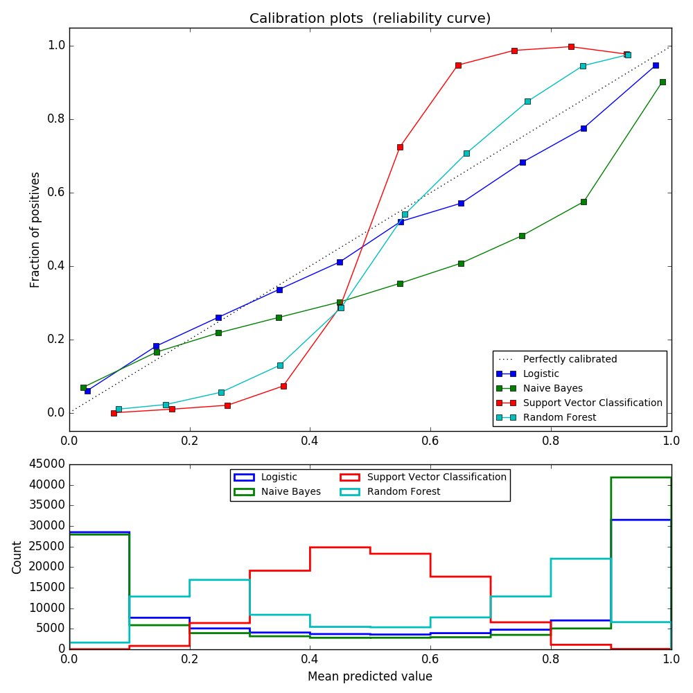
LogisticRegression () returns a properly calibrated prediction by default for direct optimization of log loss. In contrast, other methods return a biased probability. Each method has a different bias:

GaussianNB tends to push the probability to 0 or 1 (note the number of histograms). This is due to the assumption that the features are conditionally independent when given the class. This is not the case for this dataset containing two redundant features.
RandomForestClassifier shows the opposite behavior. The histogram shows peaks with a probability of about 0.2 and 0.9, and the probability of being close to 0 or 1 is very rare. This is explained by Niculescu-Mizil and Caruana [4]. "Methods of averaging predictions from the basic set of models, such as bagging and random forest, bias the predictions that the variance of the underlying base model should approach 0 or 1 from these values, so set to 0 and 1. It makes close predictions difficult. Because the predictions are limited to the interval [0,1], the error due to the variance tends to be on one side close to 0 and 1. For example, the model is relative to the case. If you need to predict p = 0, the only way bagging can achieve this is to predict zero for all buggy trees. Adding noise to a tree with averaged bagging will This noise produces a tree that predicts values greater than 0 in this case, causing the mean prediction of the background ensemble to move away from 0. Random forest-trained base-level trees are feature subsetting. This effect is most strongly observed in random forests because of its relatively large variance. " As a result, the calibration curve shows a characteristic sigmoid shape, indicating that the classifier can rely more on its "intuition" and generally return a probability close to 0 or 1.
Linear Support Vector Classification (LinearSVC) provides a larger sigmoid curve as a RandomForestClassifier. indicate. This is common with the maximum margin method (compared to Niculescu-Mizil and Caruana [4]), which focuses on hard samples near the decision boundary.

Two approaches to perform stochastic prediction calibration: a parametric approach based on Pratt's sigmoid model and an isotonic regression (sklearn.isotonic). ) Is provided as a non-parametric approach. Probabilistic calibration should be performed on new data that will not be used for model fitting. CalibratedClassifierCV The class is a model on a training sample using a cross-validation generator. Estimate each split of the parameter and calibration of the test sample. Then the expected probabilities for the fold are averaged. Already matched classifiers can be calibrated by CalibratedClassifierCV via the parameter cv =" prefit ". In this case, the user must manually note that the data for fitting and calibration of the model is discontinuous.

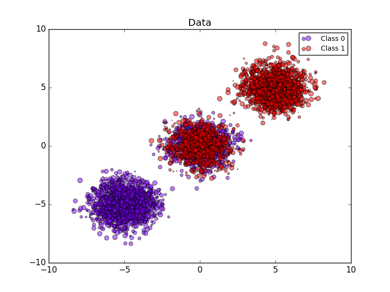
The following image shows the benefits of stochastic calibration. The first image shows two classes and three chunks of the dataset. The central chunk contains a random sample of each class. The probability of a sample of this mass should be 0.5.

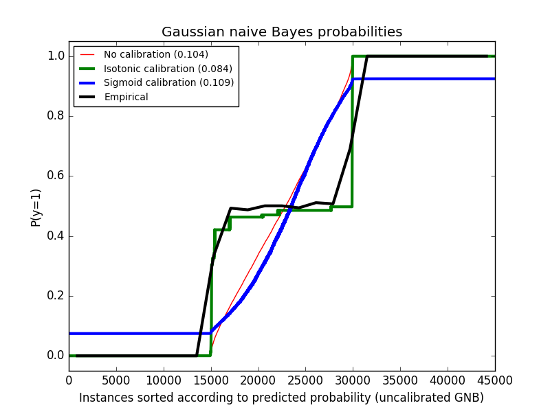
The following image shows data above estimated probabilities using an uncalibrated Gaussian naive Bayes classifier, sigmoid calibration, and nonparametric isotonic calibration. It can be observed that the nonparametric model provides the most accurate probability estimate for the central sample, 0.5.

The next experiment is performed on an artificial dataset for binary classification with 100.000 samples with 20 features (1.000 samples are used for model fitting). Of the 20 features, only 2 are useful and 10 are redundant. This figure shows the estimated probabilities obtained with a logistic regression, a linear support vector classifier (SVC), and a linear SVC with both isotonic and sigmoid calibrations. Calibration performance is assessed by the Brier score brier_score_loss and reported in the legend ( Smaller is better).

Here we can see that logistic regression is calibrated because its curves are nearly diagonal. The linear SVC calibration curve has a sigmoid curve, which is unique to "confident" classifiers. For LinearSVC, this is caused by the margin property of hinge loss. This allows the model to focus on hard samples (support vectors) near the decision boundaries. Both types of calibration solve this problem and give almost the same results. The following figure shows a Gaussian Naive Bayes calibration curve on the same data, with and without both types of calibration.

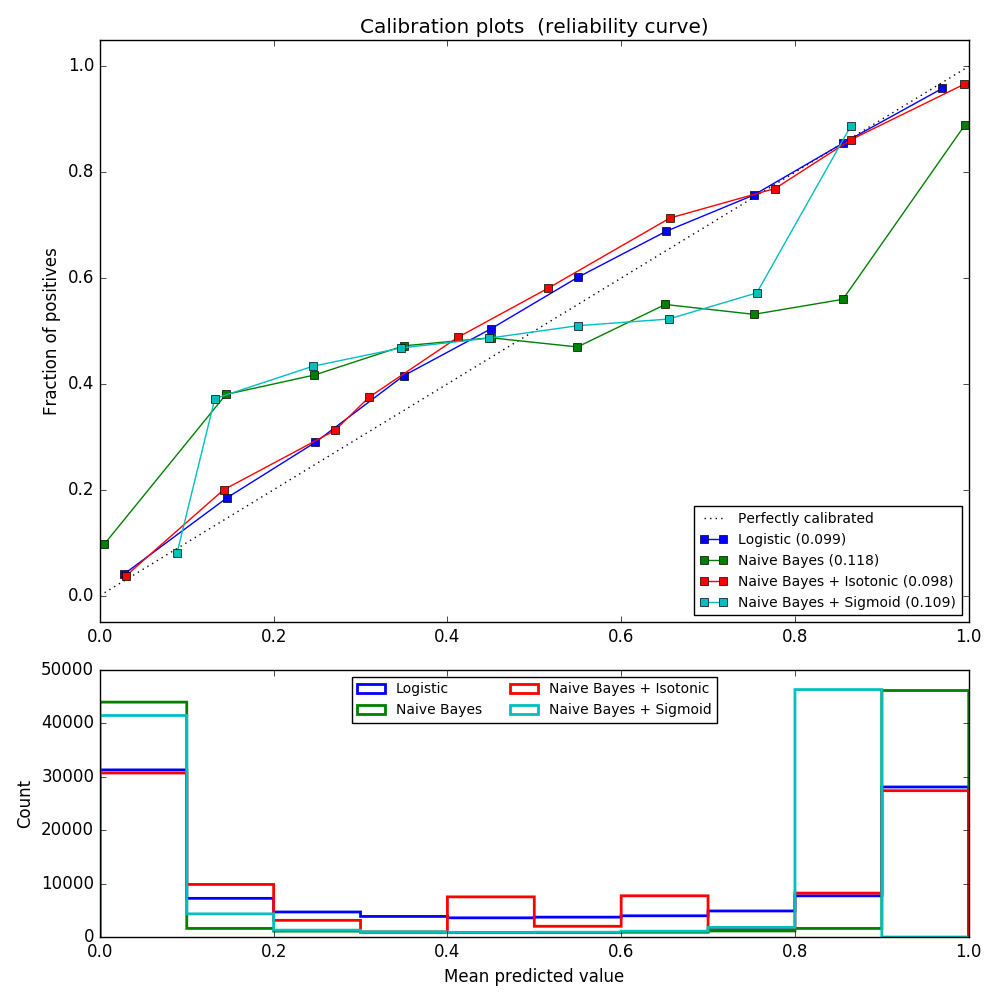
Gaussian naive Bayes gives very bad results, but it turns out to be done in ways other than linear SVC. The linear SVC shows a sigmoid calibration curve, whereas the Gaussian naive Bayes calibration curve has a transposed sigmoid shape. This is common with classifiers that are too optimistic. In this case, classifier overconfidence is caused by redundant features that violate the feature-independent naive Bayesian assumption. Gaussian naive Bayes isotonic regression probability calibration can correct this problem, as can be seen from the nearly diagonal calibration curve. Sigmoid calibration is also not as powerful as nonparametric isotonic calibration, but it improves brier scores slightly. This is an essential limitation of sigmoid calibration, and its parametric form assumes sigmoids rather than transposed sigmoid curves. However, nonparametric isotonic calibration models do not make such strong assumptions and can handle any shape with sufficient calibration data. In general, sigmoid calibration is preferred when the calibration curve is sigmoid and the calibration data is limited, but isotonic calibration is preferred in situations where a large amount of data is available for non-sigmoid calibration curves and calibration. CalibratedClassifierCV is more than one if the base estimation can. It can also handle classification tasks that include classes. In this case, the classifier is individually calibrated in a different one-to-one way for each class. When predicting the probabilities of invisible data, the calibrated probabilities for each class are predicted separately. Since their probabilities do not always match 1, post-processing is done to normalize them. The following image shows how sigmoid calibration changes the predictive probability of a three-class classification problem. An example is a standard 2 simplex with 3 corners corresponding to 3 classes. The arrows point from the random variables predicted by the uncalibrated classifier to the random variables predicted by the same classifier after the sigmoid calibration of the holdout validation set. The color indicates the true class of the instance (red: class 1, green: class 2, blue: class 3).

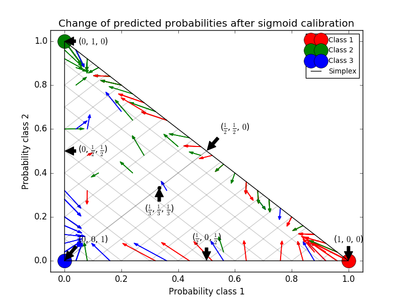
The base classifier is a random forest classifier with 25 base estimators (trees). If this classifier is trained on all 800 training data points, the predictions are overly confident and result in significant log losses. Calibrating the same classifier trained at 600 data points with method ='sigmoid' on the remaining 200 data points reduces the reliability of the prediction, ie, the edge of the simplex. Move the random variable from to the center.

This calibration results in lower log loss. Note that the alternative was to increase the number of base estimators that would result in a similar reduction in log loss.

References:
[1] Obtain calibrated probability estimates from decision trees and naive Bayes classifiers, B. Zadrozny & C. Elkan, ICML 2001
[2] Convert classifier scores to accurate multiclass probability estimates, B. Zadrozny & C. Elkan, (KDD 2002)
[3] Comparison of the probabilistic output of the support vector machine with the normalized likelihood method, J. Platt, (1999)
[4] Prediction of good probabilities by supervised learning, A. Niculescu-Mizil & R. Caruana, ICML 2005

[scikit-learn 0.18 User Guide 1. Supervised Learning](http://qiita.com/nazoking@github/items/267f2371757516f8c168#1-%E6%95%99%E5%B8%AB%E4%BB%98 From% E3% 81% 8D% E5% AD% A6% E7% BF% 92)

[PYTHON] [Translation] scikit-learn 0.18 User Guide 1.16. Probability calibration

1.16. Probability calibration