[PYTHON] Pandas User Guide "Table Formatting and PivotTables" (Official Document Japanese Translation)
This article is part of the official Pandas documentation after machine translation of the User Guide --Reshaping and pivot tables (https://pandas.pydata.org/pandas-docs/stable/user_guide/reshaping.html). It is a modification of an unnatural sentence.
If you have any mistranslations, alternative translations, questions, etc., please use the comments section or edit request.
Table shaping and pivot table
Formatting by pivoting a DataFrame object
Data is often stored in so-called "stacks" or "records".
In [1]: df
Out[1]:
         date variable     value
0  2000-01-03        A  0.469112
1  2000-01-04        A -0.282863
2  2000-01-05        A -1.509059
3  2000-01-03        B -1.135632
4  2000-01-04        B  1.212112
5  2000-01-05        B -0.173215
6  2000-01-03        C  0.119209
7  2000-01-04        C -1.044236
8  2000-01-05        C -0.861849
9  2000-01-03        D -2.104569
10 2000-01-04        D -0.494929
11 2000-01-05        D  1.071804
By the way, how to create the above DataFrame is as follows.
import pandas._testing as tm

def unpivot(frame):
    N, K = frame.shape
    data = {'value': frame.to_numpy().ravel('F'),
            'variable': np.asarray(frame.columns).repeat(N),
            'date': np.tile(np.asarray(frame.index), K)}
    return pd.DataFrame(data, columns=['date', 'variable', 'value'])


df = unpivot(tm.makeTimeDataFrame(3))
To select all rows where variable is ʻA`:
In [2]: df[df['variable'] == 'A']
Out[2]:
        date variable     value
0 2000-01-03        A  0.469112
1 2000-01-04        A -0.282863
2 2000-01-05        A -1.509059
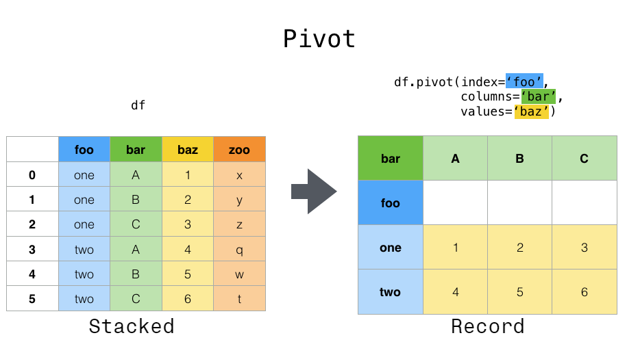
On the other hand, suppose you want to use these variables to perform time series operations. In this case, it would be better to identify the individual observations by the unique variable columns and the date ʻindex. To reshape your data into this format, [DataFrame.pivot ()](https://pandas.pydata.org/pandas-docs/stable/reference/api/pandas.DataFrame.pivot.html#pandas Use the .DataFrame.pivot) method (top-level function [pivot ()`](https://pandas.pydata.org/pandas-docs/stable/reference/api/pandas.pivot.html#pandas) .pivot) is also implemented).
In [3]: df.pivot(index='date', columns='variable', values='value')
Out[3]:
variable           A         B         C         D
date
2000-01-03  0.469112 -1.135632  0.119209 -2.104569
2000-01-04 -0.282863  1.212112 -1.044236 -0.494929
2000-01-05 -1.509059 -0.173215 -0.861849  1.071804
If the values argument is omitted and the input DataFrame has multiple columns of values that are not given to pivot as columns or indexes, the resulting" pivot " DataFrame will have the highest level of each value column. Has a Hierarchical Column (https://qiita.com/nkay/items/ Multi-Index Advanced Index) that indicates.
In [4]: df['value2'] = df['value'] * 2

In [5]: pivoted = df.pivot(index='date', columns='variable')

In [6]: pivoted
Out[6]:
               value                      ...    value2
variable           A         B         C  ...         B         C         D
date                                      ...
2000-01-03  0.469112 -1.135632  0.119209  ... -2.271265  0.238417 -4.209138
2000-01-04 -0.282863  1.212112 -1.044236  ...  2.424224 -2.088472 -0.989859
2000-01-05 -1.509059 -0.173215 -0.861849  ... -0.346429 -1.723698  2.143608

[3 rows x 8 columns]
You can then select a subset from the pivoted DataFrame.
In [7]: pivoted['value2']
Out[7]:
variable           A         B         C         D
date
2000-01-03  0.938225 -2.271265  0.238417 -4.209138
2000-01-04 -0.565727  2.424224 -2.088472 -0.989859
2000-01-05 -3.018117 -0.346429 -1.723698  2.143608
Note that if the data is isomorphic, it returns a view of the underlying data.
: ballot_box_with_check: ** Note ** If the index / column pair is not unique,
pivot ()will Raises the errorValueError: Index contains duplicate entries, cannot reshape. In this case, consider usingpivot_table ()Please give me. This is a generalization of pivots that can handle duplicate values for a single index / column pair.
Shape change by stacking and unstacking
pivot () A series closely related to the method In the method of, stack () available in Series and DataFrame # pandas.DataFrame.stack) and [ʻunstack () ](https://pandas.pydata.org/pandas-docs/stable/reference/api/pandas.DataFrame.unstack.html#pandas.DataFrame.unstack) There is a method. These methods are designed to work with the MultiIndex` object (see the chapter on Hierarchical Indexes (https://qiita.com/nkay/items/Multiindex Advanced Indexes)). The basic functions of these methods are as follows:
--stack:" Pivots "the level of the (possibly hierarchical) column label and returns a new DataFrame with that row label at the innermost level of the index.
--ʻUnstack: (reverse stacking) (probably hierarchical) row index level "pivot" to column axis to generate reconstructed DataFrame` with innermost level column label I will.
It will be easier to understand if you look at an actual example. It deals with the same dataset that we saw in the Hierarchical Index chapter.
In [8]: tuples = list(zip(*[['bar', 'bar', 'baz', 'baz',
   ...:                      'foo', 'foo', 'qux', 'qux'],
   ...:                     ['one', 'two', 'one', 'two',
   ...:                      'one', 'two', 'one', 'two']]))
   ...:

In [9]: index = pd.MultiIndex.from_tuples(tuples, names=['first', 'second'])

In [10]: df = pd.DataFrame(np.random.randn(8, 2), index=index, columns=['A', 'B'])

In [11]: df2 = df[:4]

In [12]: df2
Out[12]:
                     A         B
first second
bar   one     0.721555 -0.706771
      two    -1.039575  0.271860
baz   one    -0.424972  0.567020
      two     0.276232 -1.087401
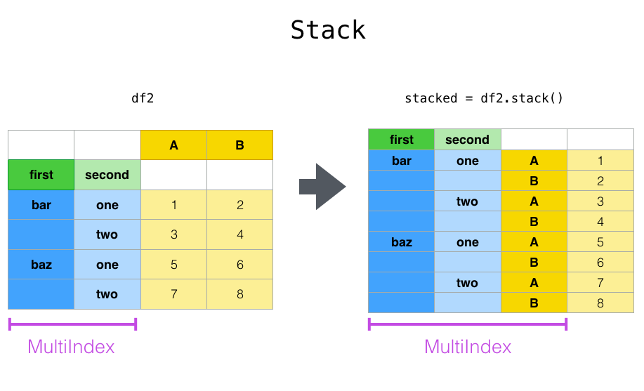
The stack function" compresses "the level of a column in DataFrame to produce one of the following:
--Series: For simple column indexes.
--DataFrame: If the column has MultiIndex.
If the column has MultiIndex, you can choose the level to stack. The stacked level will be the lowest level of the new column MultiIndex.
In [13]: stacked = df2.stack()

In [14]: stacked
Out[14]:
first  second
bar    one     A    0.721555
               B   -0.706771
       two     A   -1.039575
               B    0.271860
baz    one     A   -0.424972
               B    0.567020
       two     A    0.276232
               B   -1.087401
dtype: float64
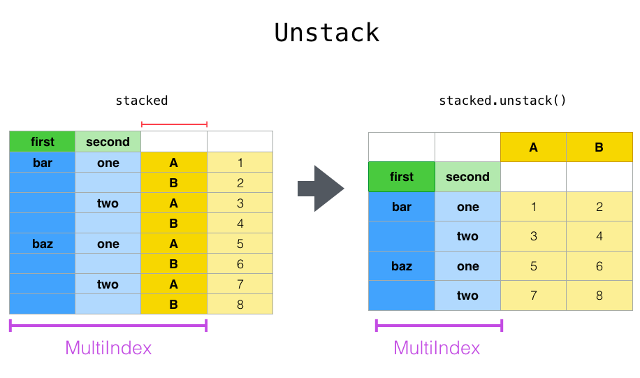
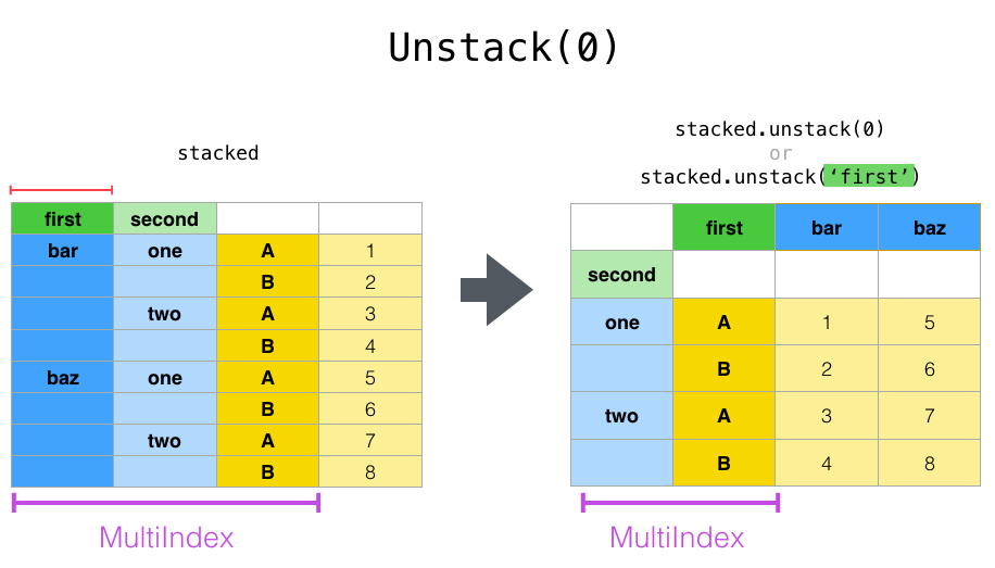
For a "stacked" DataFrame or Series (that is, ʻindex is MultiIndex), use ʻunstack to perform the opposite of stack. The default is to unstack the ** lowest level **.
In [15]: stacked.unstack()
Out[15]:
A B
first second
bar one 0.721555 -0.706771
two -1.039575 0.271860
baz one -0.424972 0.567020
two 0.276232 -1.087401
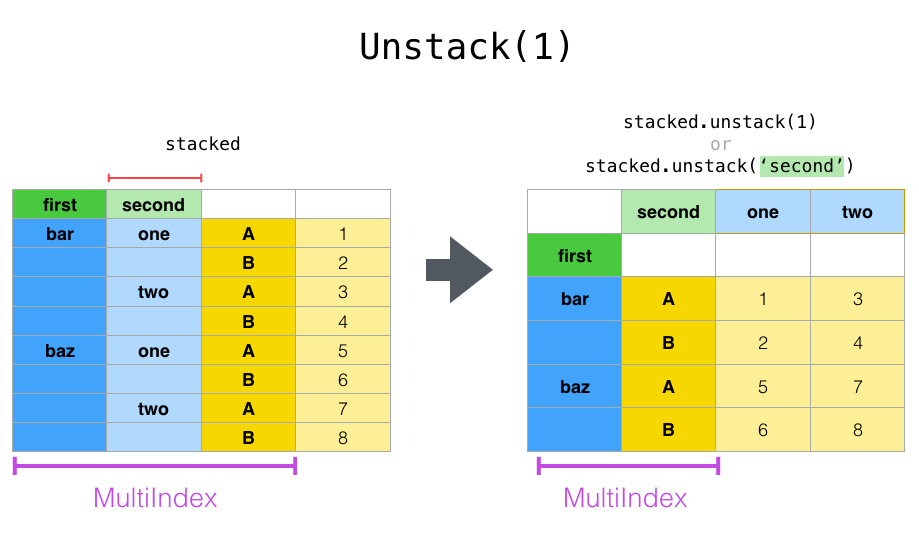
In [16]: stacked.unstack(1)
Out[16]:
second one two
first
bar A 0.721555 -1.039575
B -0.706771 0.271860
baz A -0.424972 0.276232
B 0.567020 -1.087401
In [17]: stacked.unstack(0)
Out[17]:
first bar baz
second
one A 0.721555 -0.424972
B -0.706771 0.567020
two A -1.039575 0.276232
B 0.271860 -1.087401
If the index has a name, you can use the level name instead of specifying the level number.
In [18]: stacked.unstack('second')
Out[18]:
second        one       two
first
bar   A  0.721555 -1.039575
      B -0.706771  0.271860
baz   A -0.424972  0.276232
      B  0.567020 -1.087401
Note that the stack and ʻunstackmethods implicitly sort the associated index levels. Therefore,stack and then ʻunstack (or vice versa) will return a ** sorted ** copy of the original DataFrame or Series.
In [19]: index = pd.MultiIndex.from_product([[2, 1], ['a', 'b']])

In [20]: df = pd.DataFrame(np.random.randn(4), index=index, columns=['A'])

In [21]: df
Out[21]:
            A
2 a -0.370647
  b -1.157892
1 a -1.344312
  b  0.844885

In [22]: all(df.unstack().stack() == df.sort_index())
Out[22]: True
The above code will throw a TypeError if the call to sort_index is removed.
Multiple levels
You can also stack or unstack multiple levels at once by passing a list of levels. In that case, the end result is the same as if each level in the list was processed individually.
In [23]: columns = pd.MultiIndex.from_tuples([
   ....:     ('A', 'cat', 'long'), ('B', 'cat', 'long'),
   ....:     ('A', 'dog', 'short'), ('B', 'dog', 'short')],
   ....:     names=['exp', 'animal', 'hair_length']
   ....: )
   ....:

In [24]: df = pd.DataFrame(np.random.randn(4, 4), columns=columns)

In [25]: df
Out[25]:
exp                 A         B         A         B
animal            cat       cat       dog       dog
hair_length      long      long     short     short
0            1.075770 -0.109050  1.643563 -1.469388
1            0.357021 -0.674600 -1.776904 -0.968914
2           -1.294524  0.413738  0.276662 -0.472035
3           -0.013960 -0.362543 -0.006154 -0.923061

In [26]: df.stack(level=['animal', 'hair_length'])
Out[26]:
exp                          A         B
  animal hair_length
0 cat    long         1.075770 -0.109050
  dog    short        1.643563 -1.469388
1 cat    long         0.357021 -0.674600
  dog    short       -1.776904 -0.968914
2 cat    long        -1.294524  0.413738
  dog    short        0.276662 -0.472035
3 cat    long        -0.013960 -0.362543
  dog    short       -0.006154 -0.923061
The list of levels can contain either level names or level numbers (although the two cannot be mixed).
# df.stack(level=['animal', 'hair_length'])
#This code is equal to
In [27]: df.stack(level=[1, 2])
Out[27]:
exp                          A         B
  animal hair_length
0 cat    long         1.075770 -0.109050
  dog    short        1.643563 -1.469388
1 cat    long         0.357021 -0.674600
  dog    short       -1.776904 -0.968914
2 cat    long        -1.294524  0.413738
  dog    short        0.276662 -0.472035
3 cat    long        -0.013960 -0.362543
  dog    short       -0.006154 -0.923061
Missing data
These functions are also flexible in handling missing data and will work even if each subgroup in the hierarchical index does not have the same set of labels. You can also handle unsorted indexes (of course, you can sort by calling sort_index). Here is a more complex example:
In [28]: columns = pd.MultiIndex.from_tuples([('A', 'cat'), ('B', 'dog'),
   ....:                                      ('B', 'cat'), ('A', 'dog')],
   ....:                                     names=['exp', 'animal'])
   ....:

In [29]: index = pd.MultiIndex.from_product([('bar', 'baz', 'foo', 'qux'),
   ....:                                     ('one', 'two')],
   ....:                                    names=['first', 'second'])
   ....:

In [30]: df = pd.DataFrame(np.random.randn(8, 4), index=index, columns=columns)

In [31]: df2 = df.iloc[[0, 1, 2, 4, 5, 7]]

In [32]: df2
Out[32]:
exp                  A         B                   A
animal             cat       dog       cat       dog
first second
bar   one     0.895717  0.805244 -1.206412  2.565646
      two     1.431256  1.340309 -1.170299 -0.226169
baz   one     0.410835  0.813850  0.132003 -0.827317
foo   one    -1.413681  1.607920  1.024180  0.569605
      two     0.875906 -2.211372  0.974466 -2.006747
qux   two    -1.226825  0.769804 -1.281247 -0.727707
As mentioned earlier, you can call stack with the level argument to choose which level in the column to stack.
In [33]: df2.stack('exp')
Out[33]:
animal                 cat       dog
first second exp
bar   one    A    0.895717  2.565646
             B   -1.206412  0.805244
      two    A    1.431256 -0.226169
             B   -1.170299  1.340309
baz   one    A    0.410835 -0.827317
             B    0.132003  0.813850
foo   one    A   -1.413681  0.569605
             B    1.024180  1.607920
      two    A    0.875906 -2.006747
             B    0.974466 -2.211372
qux   two    A   -1.226825 -0.727707
             B   -1.281247  0.769804

In [34]: df2.stack('animal')
Out[34]:
exp                         A         B
first second animal
bar   one    cat     0.895717 -1.206412
             dog     2.565646  0.805244
      two    cat     1.431256 -1.170299
             dog    -0.226169  1.340309
baz   one    cat     0.410835  0.132003
             dog    -0.827317  0.813850
foo   one    cat    -1.413681  1.024180
             dog     0.569605  1.607920
      two    cat     0.875906  0.974466
             dog    -2.006747 -2.211372
qux   two    cat    -1.226825 -1.281247
             dog    -0.727707  0.769804
If the subgroups do not have the same set of labels, unstacking can cause missing values. By default, missing values are replaced with the default fill-in-the-blank values for that data type (such as NaN for floats, NaT for datetime-like). For integer types, the data is converted to float by default and the missing value is set to NaN.
In [35]: df3 = df.iloc[[0, 1, 4, 7], [1, 2]]

In [36]: df3
Out[36]:
exp                  B
animal             dog       cat
first second
bar   one     0.805244 -1.206412
      two     1.340309 -1.170299
foo   one     1.607920  1.024180
qux   two     0.769804 -1.281247

In [37]: df3.unstack()
Out[37]:
exp            B
animal       dog                 cat
second       one       two       one       two
first
bar     0.805244  1.340309 -1.206412 -1.170299
foo     1.607920       NaN  1.024180       NaN
qux          NaN  0.769804       NaN -1.281247
ʻUnstack can also take an optional fill_value` argument that specifies the value of the missing data.
In [38]: df3.unstack(fill_value=-1e9)
Out[38]:
exp                B
animal           dog                         cat
second           one           two           one           two
first
bar     8.052440e-01  1.340309e+00 -1.206412e+00 -1.170299e+00
foo     1.607920e+00 -1.000000e+09  1.024180e+00 -1.000000e+09
qux    -1.000000e+09  7.698036e-01 -1.000000e+09 -1.281247e+00
For MultiIndex
Even when the column is MultiIndex, it can be unstacked without any problems.
In [39]: df[:3].unstack(0)
Out[39]:
exp            A                   B  ...                   A
animal       cat                 dog  ...       cat       dog
first        bar       baz       bar  ...       baz       bar       baz
second                                ...
one     0.895717  0.410835  0.805244  ...  0.132003  2.565646 -0.827317
two     1.431256       NaN  1.340309  ...       NaN -0.226169       NaN

[2 rows x 8 columns]

In [40]: df2.unstack(1)
Out[40]:
exp            A                   B  ...                   A
animal       cat                 dog  ...       cat       dog
second       one       two       one  ...       two       one       two
first                                 ...
bar     0.895717  1.431256  0.805244  ... -1.170299  2.565646 -0.226169
baz     0.410835       NaN  0.813850  ...       NaN -0.827317       NaN
foo    -1.413681  0.875906  1.607920  ...  0.974466  0.569605 -2.006747
qux          NaN -1.226825       NaN  ... -1.281247       NaN -0.727707

[4 rows x 8 columns]
Plastic surgery by melt
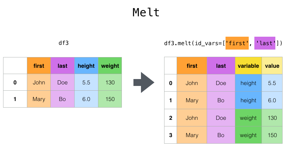
Top-level melt () functions and their corresponding DataFrame. melt () has one or more DataFrame Converts to an "unpivoted" state where the column of is regarded as a * identification variable * and all other columns are regarded as * measured variables *, leaving only two non-identifying columns, "variable" and "value". Useful for. The names of the remaining columns can be customized by specifying the var_name and value_name parameters.
For example
In [41]: cheese = pd.DataFrame({'first': ['John', 'Mary'],
   ....:                        'last': ['Doe', 'Bo'],
   ....:                        'height': [5.5, 6.0],
   ....:                        'weight': [130, 150]})
   ....:

In [42]: cheese
Out[42]:
  first last  height  weight
0  John  Doe     5.5     130
1  Mary   Bo     6.0     150

In [43]: cheese.melt(id_vars=['first', 'last'])
Out[43]:
  first last variable  value
0  John  Doe   height    5.5
1  Mary   Bo   height    6.0
2  John  Doe   weight  130.0
3  Mary   Bo   weight  150.0

In [44]: cheese.melt(id_vars=['first', 'last'], var_name='quantity')
Out[44]:
  first last quantity  value
0  John  Doe   height    5.5
1  Mary   Bo   height    6.0
2  John  Doe   weight  130.0
3  Mary   Bo   weight  150.0
As another conversion method, wide_to_long () is useful for panel data. It is a function. Less flexible than melt (), but more user It's friendly.
In [45]: dft = pd.DataFrame({"A1970": {0: "a", 1: "b", 2: "c"},
   ....:                     "A1980": {0: "d", 1: "e", 2: "f"},
   ....:                     "B1970": {0: 2.5, 1: 1.2, 2: .7},
   ....:                     "B1980": {0: 3.2, 1: 1.3, 2: .1},
   ....:                     "X": dict(zip(range(3), np.random.randn(3)))
   ....:                    })
   ....:

In [46]: dft["id"] = dft.index

In [47]: dft
Out[47]:
  A1970 A1980  B1970  B1980         X  id
0     a     d    2.5    3.2 -0.121306   0
1     b     e    1.2    1.3 -0.097883   1
2     c     f    0.7    0.1  0.695775   2

In [48]: pd.wide_to_long(dft, ["A", "B"], i="id", j="year")
Out[48]:
                X  A    B
id year
0  1970 -0.121306  a  2.5
1  1970 -0.097883  b  1.2
2  1970  0.695775  c  0.7
0  1980 -0.121306  d  3.2
1  1980 -0.097883  e  1.3
2  1980  0.695775  f  0.1
Combination with statistics and GroupBy
You should be aware that combining pivot, stack, and ʻunstack` with GroupBy and basic Series and DataFrame statistical functions allows for very expressive and fast data manipulation.
In [49]: df
Out[49]:
exp                  A         B                   A
animal             cat       dog       cat       dog
first second
bar   one     0.895717  0.805244 -1.206412  2.565646
      two     1.431256  1.340309 -1.170299 -0.226169
baz   one     0.410835  0.813850  0.132003 -0.827317
      two    -0.076467 -1.187678  1.130127 -1.436737
foo   one    -1.413681  1.607920  1.024180  0.569605
      two     0.875906 -2.211372  0.974466 -2.006747
qux   one    -0.410001 -0.078638  0.545952 -1.219217
      two    -1.226825  0.769804 -1.281247 -0.727707

In [50]: df.stack().mean(1).unstack()
Out[50]:
animal             cat       dog
first second
bar   one    -0.155347  1.685445
      two     0.130479  0.557070
baz   one     0.271419 -0.006733
      two     0.526830 -1.312207
foo   one    -0.194750  1.088763
      two     0.925186 -2.109060
qux   one     0.067976 -0.648927
      two    -1.254036  0.021048

#Similar results in another way
In [51]: df.groupby(level=1, axis=1).mean()
Out[51]:
animal             cat       dog
first second
bar   one    -0.155347  1.685445
      two     0.130479  0.557070
baz   one     0.271419 -0.006733
      two     0.526830 -1.312207
foo   one    -0.194750  1.088763
      two     0.925186 -2.109060
qux   one     0.067976 -0.648927
      two    -1.254036  0.021048

In [52]: df.stack().groupby(level=1).mean()
Out[52]:
exp            A         B
second
one     0.071448  0.455513
two    -0.424186 -0.204486

In [53]: df.mean().unstack(0)
Out[53]:
exp            A         B
animal
cat     0.060843  0.018596
dog    -0.413580  0.232430
Pivot table
pivot () has different data types (strings) , Numeric, etc.), but pandas provides pivot_table () for pivoting by aggregating numerical data. api / pandas.pivot_table.html # pandas.pivot_table) is also provided.
Spreadsheet-style pivot table using the function pivot_table () Can be created. See Cookbook for more advanced operations.
It takes some arguments.
--data: DataFrame object.
--value: A column or list of columns to aggregate.
--ʻIndex: Column, Grouper, array of the same length as the data, or a list of them. Keys to group by index in the pivot table. If an array is passed, it will be aggregated in the same way as the column values. --columns: An array of the same length as the columns, Grouper, or data, or a list of them. Keys to group by columns in the PivotTable. If an array is passed, it will be aggregated in the same way as the column values. --ʻAggfunc: Function used for aggregation. The default is numpy.mean.
Consider the following dataset.
In [54]: import datetime

In [55]: df = pd.DataFrame({'A': ['one', 'one', 'two', 'three'] * 6,
   ....:                    'B': ['A', 'B', 'C'] * 8,
   ....:                    'C': ['foo', 'foo', 'foo', 'bar', 'bar', 'bar'] * 4,
   ....:                    'D': np.random.randn(24),
   ....:                    'E': np.random.randn(24),
   ....:                    'F': [datetime.datetime(2013, i, 1) for i in range(1, 13)]
   ....:                    + [datetime.datetime(2013, i, 15) for i in range(1, 13)]})
   ....:

In [56]: df
Out[56]:
        A  B    C         D         E          F
0     one  A  foo  0.341734 -0.317441 2013-01-01
1     one  B  foo  0.959726 -1.236269 2013-02-01
2     two  C  foo -1.110336  0.896171 2013-03-01
3   three  A  bar -0.619976 -0.487602 2013-04-01
4     one  B  bar  0.149748 -0.082240 2013-05-01
..    ... ..  ...       ...       ...        ...
19  three  B  foo  0.690579 -2.213588 2013-08-15
20    one  C  foo  0.995761  1.063327 2013-09-15
21    one  A  bar  2.396780  1.266143 2013-10-15
22    two  B  bar  0.014871  0.299368 2013-11-15
23  three  C  bar  3.357427 -0.863838 2013-12-15

[24 rows x 6 columns]
It's very easy to create a PivotTable from this data.
In [57]: pd.pivot_table(df, values='D', index=['A', 'B'], columns=['C'])
Out[57]:
C             bar       foo
A     B
one   A  1.120915 -0.514058
      B -0.338421  0.002759
      C -0.538846  0.699535
three A -1.181568       NaN
      B       NaN  0.433512
      C  0.588783       NaN
two   A       NaN  1.000985
      B  0.158248       NaN
      C       NaN  0.176180

In [58]: pd.pivot_table(df, values='D', index=['B'], columns=['A', 'C'], aggfunc=np.sum)
Out[58]:
A       one               three                 two
C       bar       foo       bar       foo       bar       foo
B
A  2.241830 -1.028115 -2.363137       NaN       NaN  2.001971
B -0.676843  0.005518       NaN  0.867024  0.316495       NaN
C -1.077692  1.399070  1.177566       NaN       NaN  0.352360

In [59]: pd.pivot_table(df, values=['D', 'E'], index=['B'], columns=['A', 'C'],
   ....:                aggfunc=np.sum)
   ....:
Out[59]:
          D                      ...         E
A       one               three  ...     three       two
C       bar       foo       bar  ...       foo       bar       foo
B                                ...
A  2.241830 -1.028115 -2.363137  ...       NaN       NaN  0.128491
B -0.676843  0.005518       NaN  ... -2.128743 -0.194294       NaN
C -1.077692  1.399070  1.177566  ...       NaN       NaN  0.872482

[3 rows x 12 columns]
The result object is a DataFrame that probably has a hierarchical index on the rows and columns. If no column name is specified for values, the PivotTable will add a hierarchy level to the column to contain all the data that can be aggregated.
In [60]: pd.pivot_table(df, index=['A', 'B'], columns=['C'])
Out[60]:
                D                   E
C             bar       foo       bar       foo
A     B
one   A  1.120915 -0.514058  1.393057 -0.021605
      B -0.338421  0.002759  0.684140 -0.551692
      C -0.538846  0.699535 -0.988442  0.747859
three A -1.181568       NaN  0.961289       NaN
      B       NaN  0.433512       NaN -1.064372
      C  0.588783       NaN -0.131830       NaN
two   A       NaN  1.000985       NaN  0.064245
      B  0.158248       NaN -0.097147       NaN
      C       NaN  0.176180       NaN  0.436241
You can also use Grouper for the ʻindex and columnsarguments. For more information onGrouper`, see Grouping with Grouper (https://pandas.pydata.org/pandas-docs/stable/user_guide/groupby.html#groupby-specify).
In [61]: pd.pivot_table(df, values='D', index=pd.Grouper(freq='M', key='F'),
   ....:                columns='C')
   ....:
Out[61]:
C                bar       foo
F
2013-01-31       NaN -0.514058
2013-02-28       NaN  0.002759
2013-03-31       NaN  0.176180
2013-04-30 -1.181568       NaN
2013-05-31 -0.338421       NaN
2013-06-30 -0.538846       NaN
2013-07-31       NaN  1.000985
2013-08-31       NaN  0.433512
2013-09-30       NaN  0.699535
2013-10-31  1.120915       NaN
2013-11-30  0.158248       NaN
2013-12-31  0.588783       NaN
You can beautifully render the output of a table with missing values omitted by calling to_string as needed.
In [62]: table = pd.pivot_table(df, index=['A', 'B'], columns=['C'])

In [63]: print(table.to_string(na_rep=''))
                D                   E
C             bar       foo       bar       foo
A     B
one   A  1.120915 -0.514058  1.393057 -0.021605
      B -0.338421  0.002759  0.684140 -0.551692
      C -0.538846  0.699535 -0.988442  0.747859
three A -1.181568            0.961289
      B            0.433512           -1.064372
      C  0.588783           -0.131830
two   A            1.000985            0.064245
      B  0.158248           -0.097147
      C            0.176180            0.436241
** pivot_table can also be used as an instance method of DataFrame. ** **
⇒ DataFrame.pivot_table()。
Add subtotal
Passing margins = True to pivot_table adds a special column and row called ʻAll` that aggregates the entire row and column category for each group.
Cross tabulation
Using crosstab (), you can use two (or more) You can cross-tabulate elements. If no array of values and aggregate function are passed, by default crosstab will calculate the frequency table of the elements.
It also receives the following arguments:
--ʻIndex: Array etc. Values to group by row. --columns: Array etc. Values to group by column. --values: Array etc. Optional. An array of values to aggregate according to the element. --ʻAggfunc: Function. Optional. If omitted, the frequency table is calculated.
--rownames: Sequence. The default is None. Must match the number of row arrays passed (the length of the array passed in the ʻindex argument). --colnames: Sequence. The default is None. Must match the number of column arrays passed (the length of the array passed in the columns argument). --margins: Boolean value. The default is False. Add subtotals to rows and columns. --normalizeBoolean value ・ {‘all’, ‘index’, ‘columns’} ・ {0,1}. The default isFalse`. Normalize by dividing all values by the sum of the values.
Unless a row or column name is specified in the crosstab, the name attribute of each passed Series is used.
For example
In [65]: foo, bar, dull, shiny, one, two = 'foo', 'bar', 'dull', 'shiny', 'one', 'two'

In [66]: a = np.array([foo, foo, bar, bar, foo, foo], dtype=object)

In [67]: b = np.array([one, one, two, one, two, one], dtype=object)

In [68]: c = np.array([dull, dull, shiny, dull, dull, shiny], dtype=object)

In [69]: pd.crosstab(a, [b, c], rownames=['a'], colnames=['b', 'c'])
Out[69]:
b    one        two
c   dull shiny dull shiny
a
bar    1     0    0     1
foo    2     1    1     0
If crosstab receives only two Series, a frequency table is returned.
In [70]: df = pd.DataFrame({'A': [1, 2, 2, 2, 2], 'B': [3, 3, 4, 4, 4],
   ....:                    'C': [1, 1, np.nan, 1, 1]})
   ....:

In [71]: df
Out[71]:
   A  B    C
0  1  3  1.0
1  2  3  1.0
2  2  4  NaN
3  2  4  1.0
4  2  4  1.0

In [72]: pd.crosstab(df['A'], df['B'])
Out[72]:
B  3  4
A
1  1  0
2  1  3
If the data passed has Categorical data, then the ** all ** categories will be included in the crosstab, even if the actual data does not contain instances of a particular category.
In [73]: foo = pd.Categorical(['a', 'b'], categories=['a', 'b', 'c'])

In [74]: bar = pd.Categorical(['d', 'e'], categories=['d', 'e', 'f'])

In [75]: pd.crosstab(foo, bar)
Out[75]:
col_0  d  e
row_0
a      1  0
b      0  1
Normalization
The frequency table can also be normalized to display percentages instead of counts using the normalize argument.
In [76]: pd.crosstab(df['A'], df['B'], normalize=True)
Out[76]:
B    3    4
A
1  0.2  0.0
2  0.2  0.6
normalize can also be normalized for each row or column.
In [77]: pd.crosstab(df['A'], df['B'], normalize='columns')
Out[77]:
B    3    4
A
1  0.5  0.0
2  0.5  1.0
If you pass the third Series and the aggregate function (ʻaggfunc) to crosstab, the function for the value in the third Series of each group defined in the first two Series`s. Is applied.
In [78]: pd.crosstab(df['A'], df['B'], values=df['C'], aggfunc=np.sum)
Out[78]:
B    3    4
A
1  1.0  NaN
2  1.0  2.0
Add subtotal
Finally, you can add subtotals and normalize their output.
In [79]: pd.crosstab(df['A'], df['B'], values=df['C'], aggfunc=np.sum, normalize=True,
   ....:             margins=True)
   ....:
Out[79]:
B       3    4   All
A
1    0.25  0.0  0.25
2    0.25  0.5  0.75
All  0.50  0.5  1.00
Binning
The cut () function performs grouping calculations for input array values. I will do it. It is often used to convert continuous variables to discrete or categorical variables.
In [80]: ages = np.array([10, 15, 13, 12, 23, 25, 28, 59, 60])

In [81]: pd.cut(ages, bins=3)
Out[81]:
[(9.95, 26.667], (9.95, 26.667], (9.95, 26.667], (9.95, 26.667], (9.95, 26.667], (9.95, 26.667], (26.667, 43.333], (43.333, 60.0], (43.333, 60.0]]
Categories (3, interval[float64]): [(9.95, 26.667] < (26.667, 43.333] < (43.333, 60.0]]
Passing an integer as the bins argument will form a monospaced bin. You can also specify a custom bin edge.
In [82]: c = pd.cut(ages, bins=[0, 18, 35, 70])

In [83]: c
Out[83]:
[(0, 18], (0, 18], (0, 18], (0, 18], (18, 35], (18, 35], (18, 35], (35, 70], (35, 70]]
Categories (3, interval[int64]): [(0, 18] < (18, 35] < (35, 70]]
If you pass ʻIntervalIndex to the bins` argument, it will be used to bin the data.
pd.cut([25, 20, 50], bins=c.categories)
Calculation of indicator variables and dummy variables
Using get_dummies () makes categorical variables "dummy" and "markers" Can be converted to DataFrame. For example, from a DataFrame column (Series) with k different values, you can create a DataFrame containing k columns consisting of 1s and 0s.
In [84]: df = pd.DataFrame({'key': list('bbacab'), 'data1': range(6)})

In [85]: pd.get_dummies(df['key'])
Out[85]:
   a  b  c
0  0  1  0
1  0  1  0
2  1  0  0
3  0  0  1
4  1  0  0
5  0  1  0
Prefixing column names is useful, for example, when merging the result with the original DataFrame.
In [86]: dummies = pd.get_dummies(df['key'], prefix='key')

In [87]: dummies
Out[87]:
   key_a  key_b  key_c
0      0      1      0
1      0      1      0
2      1      0      0
3      0      0      1
4      1      0      0
5      0      1      0

In [88]: df[['data1']].join(dummies)
Out[88]:
   data1  key_a  key_b  key_c
0      0      0      1      0
1      1      0      1      0
2      2      1      0      0
3      3      0      0      1
4      4      1      0      0
5      5      0      1      0
This function is often used with discretized functions like cut.
In [89]: values = np.random.randn(10)

In [90]: values
Out[90]:
array([ 0.4082, -1.0481, -0.0257, -0.9884,  0.0941,  1.2627,  1.29  ,
        0.0824, -0.0558,  0.5366])

In [91]: bins = [0, 0.2, 0.4, 0.6, 0.8, 1]

In [92]: pd.get_dummies(pd.cut(values, bins))
Out[92]:
   (0.0, 0.2]  (0.2, 0.4]  (0.4, 0.6]  (0.6, 0.8]  (0.8, 1.0]
0           0           0           1           0           0
1           0           0           0           0           0
2           0           0           0           0           0
3           0           0           0           0           0
4           1           0           0           0           0
5           0           0           0           0           0
6           0           0           0           0           0
7           1           0           0           0           0
8           0           0           0           0           0
9           0           0           1           0           0
See also Series.str.get_dummies Please give me.
get_dummies () can also receive DataFrame. By default, all categorical variables (in the statistical sense, that is, those with * object * or * categorical * data types) are encoded into dummy variables.
In [93]: df = pd.DataFrame({'A': ['a', 'b', 'a'], 'B': ['c', 'c', 'b'],
   ....:                    'C': [1, 2, 3]})
   ....:

In [94]: pd.get_dummies(df)
Out[94]:
   C  A_a  A_b  B_b  B_c
0  1    1    0    0    1
1  2    0    1    0    1
2  3    1    0    1    0
All non-object columns are included in the output as is. You can control which columns are encoded with the columns argument.
In [95]: pd.get_dummies(df, columns=['A'])
Out[95]:
   B  C  A_a  A_b
0  c  1    1    0
1  c  2    0    1
2  b  3    1    0
You can see that the B column is still included in the output, but it is not encoded. If you don't want to include it in the output, drop B before calling get_dummies.
As with the Series version, you can pass the values for prefix and prefix_sep. By default, the column name is used as the prefix and "_" is used as the column name delimiter. prefix and prefix_sep can be specified in the following three ways.
--String: Use the same value for the prefix or prefix_sep of each column to encode.
--List: Must be as long as the number of columns to be encoded.
--Dictionary: Map column names to prefixes.
In [96]: simple = pd.get_dummies(df, prefix='new_prefix')

In [97]: simple
Out[97]:
   C  new_prefix_a  new_prefix_b  new_prefix_b  new_prefix_c
0  1             1             0             0             1
1  2             0             1             0             1
2  3             1             0             1             0

In [98]: from_list = pd.get_dummies(df, prefix=['from_A', 'from_B'])

In [99]: from_list
Out[99]:
   C  from_A_a  from_A_b  from_B_b  from_B_c
0  1         1         0         0         1
1  2         0         1         0         1
2  3         1         0         1         0

In [100]: from_dict = pd.get_dummies(df, prefix={'B': 'from_B', 'A': 'from_A'})

In [101]: from_dict
Out[101]:
   C  from_A_a  from_A_b  from_B_b  from_B_c
0  1         1         0         0         1
1  2         0         1         0         1
2  3         1         0         1         0
To avoid collinearity when using the results in a statistical model, it may be useful to keep only the k-1 level of the categorical variable. You can switch to this mode using drop_first.
In [102]: s = pd.Series(list('abcaa'))

In [103]: pd.get_dummies(s)
Out[103]:
   a  b  c
0  1  0  0
1  0  1  0
2  0  0  1
3  1  0  0
4  1  0  0

In [104]: pd.get_dummies(s, drop_first=True)
Out[104]:
   b  c
0  0  0
1  1  0
2  0  1
3  0  0
4  0  0
If the column contains only one level, it will be omitted in the result.
In [105]: df = pd.DataFrame({'A': list('aaaaa'), 'B': list('ababc')})

In [106]: pd.get_dummies(df)
Out[106]:
   A_a  B_a  B_b  B_c
0    1    1    0    0
1    1    0    1    0
2    1    1    0    0
3    1    0    1    0
4    1    0    0    1

In [107]: pd.get_dummies(df, drop_first=True)
Out[107]:
   B_b  B_c
0    0    0
1    1    0
2    0    0
3    1    0
4    0    1
By default, the new column will be np.uint8dtype. Use the dtype argument to select a different data type.
In [108]: df = pd.DataFrame({'A': list('abc'), 'B': [1.1, 2.2, 3.3]})

In [109]: pd.get_dummies(df, dtype=bool).dtypes
Out[109]:
B      float64
A_a       bool
A_b       bool
A_c       bool
dtype: object
_ From version 0.23.0 _
Element value (label encoding)
To encode a one-dimensional value as an enum, factorize ()Use the.
In [110]: x = pd.Series(['A', 'A', np.nan, 'B', 3.14, np.inf])

In [111]: x
Out[111]:
0       A
1       A
2     NaN
3       B
4    3.14
5     inf
dtype: object

In [112]: labels, uniques = pd.factorize(x)

In [113]: labels
Out[113]: array([ 0,  0, -1,  1,  2,  3])

In [114]: uniques
Out[114]: Index(['A', 'B', 3.14, inf], dtype='object')
Note that factorize is similar to numpy.unique, but handles NaN differently.
: ballot_box_with_check: ** Note ** The following
numpy.uniquefails withTypeErrorin Python 3 due to an alignment bug. For more information, please see here.
In [1]: x = pd.Series(['A', 'A', np.nan, 'B', 3.14, np.inf])
In [2]: pd.factorize(x, sort=True)
Out[2]:
(array([ 2,  2, -1,  3,  0,  1]),
 Index([3.14, inf, 'A', 'B'], dtype='object'))

In [3]: np.unique(x, return_inverse=True)[::-1]
Out[3]: (array([3, 3, 0, 4, 1, 2]), array([nan, 3.14, inf, 'A', 'B'], dtype=object))
: ballot_box_with_check: ** Note ** If you want to treat a column as a categorical variable (like R factor),
df ["cat_col"] = pd.Categorical (df ["col"])ordf ["cat_col"] = You can use df ["col"] .astype ("category"). For complete documentation onCategorical, see Introduction to Categorical //pandas.pydata.org/pandas-docs/stable/user_guide/categorical.html#categorical) and API Documentation See # api-arrays-categorical).
Example
This section contains frequently asked questions and examples. The column names and associated column values have names that correspond to how this DataFrame is pivoted in the answers below.
In [115]: np.random.seed([3, 1415])

In [116]: n = 20

In [117]: cols = np.array(['key', 'row', 'item', 'col'])

In [118]: df = cols + pd.DataFrame((np.random.randint(5, size=(n, 4))
   .....:                          // [2, 1, 2, 1]).astype(str))
   .....:

In [119]: df.columns = cols

In [120]: df = df.join(pd.DataFrame(np.random.rand(n, 2).round(2)).add_prefix('val'))

In [121]: df
Out[121]:
     key   row   item   col  val0  val1
0   key0  row3  item1  col3  0.81  0.04
1   key1  row2  item1  col2  0.44  0.07
2   key1  row0  item1  col0  0.77  0.01
3   key0  row4  item0  col2  0.15  0.59
4   key1  row0  item2  col1  0.81  0.64
..   ...   ...    ...   ...   ...   ...
15  key0  row3  item1  col1  0.31  0.23
16  key0  row0  item2  col3  0.86  0.01
17  key0  row4  item0  col3  0.64  0.21
18  key2  row2  item2  col0  0.13  0.45
19  key0  row2  item0  col4  0.37  0.70

[20 rows x 6 columns]
Pivot with a single aggregate
Suppose you want to pivot df so that the value of col is the column, the value of row is the index, and the average of val0 is the table value. At this time, the resulting DataFrame looks like this:
col   col0   col1   col2   col3  col4
row
row0  0.77  0.605    NaN  0.860  0.65
row2  0.13    NaN  0.395  0.500  0.25
row3   NaN  0.310    NaN  0.545   NaN
row4   NaN  0.100  0.395  0.760  0.24
To find this, use pivot_table (). Note that ʻaggfunc ='mean'` is the default behavior, although explicitly mentioned here.
In [122]: df.pivot_table(
   .....:     values='val0', index='row', columns='col', aggfunc='mean')
   .....:
Out[122]:
col   col0   col1   col2   col3  col4
row
row0  0.77  0.605    NaN  0.860  0.65
row2  0.13    NaN  0.395  0.500  0.25
row3   NaN  0.310    NaN  0.545   NaN
row4   NaN  0.100  0.395  0.760  0.24
You can also use the fill_value parameter to replace missing values.
In [123]: df.pivot_table(
   .....:     values='val0', index='row', columns='col', aggfunc='mean', fill_value=0)
   .....:
Out[123]:
col   col0   col1   col2   col3  col4
row
row0  0.77  0.605  0.000  0.860  0.65
row2  0.13  0.000  0.395  0.500  0.25
row3  0.00  0.310  0.000  0.545  0.00
row4  0.00  0.100  0.395  0.760  0.24
Also, be aware that you can pass other aggregate functions. For example, you can pass sum.
In [124]: df.pivot_table(
   .....:     values='val0', index='row', columns='col', aggfunc='sum', fill_value=0)
   .....:
Out[124]:
col   col0  col1  col2  col3  col4
row
row0  0.77  1.21  0.00  0.86  0.65
row2  0.13  0.00  0.79  0.50  0.50
row3  0.00  0.31  0.00  1.09  0.00
row4  0.00  0.10  0.79  1.52  0.24
Another aggregation is to calculate how often columns and rows occur at the same time (called "cross aggregation"). To do this, pass size to the ʻaggfunc` parameter.
In [125]: df.pivot_table(index='row', columns='col', fill_value=0, aggfunc='size')
Out[125]:
col   col0  col1  col2  col3  col4
row
row0     1     2     0     1     1
row2     1     0     2     1     2
row3     0     1     0     2     0
row4     0     1     2     2     1
Pivot with multiple aggregates
You can also perform multiple aggregations. For example, you can pass a list to the ʻaggfunc argument to perform both the sum and the mean mean.
In [126]: df.pivot_table(
   .....:     values='val0', index='row', columns='col', aggfunc=['mean', 'sum'])
   .....:
Out[126]:
      mean                              sum
col   col0   col1   col2   col3  col4  col0  col1  col2  col3  col4
row
row0  0.77  0.605    NaN  0.860  0.65  0.77  1.21   NaN  0.86  0.65
row2  0.13    NaN  0.395  0.500  0.25  0.13   NaN  0.79  0.50  0.50
row3   NaN  0.310    NaN  0.545   NaN   NaN  0.31   NaN  1.09   NaN
row4   NaN  0.100  0.395  0.760  0.24   NaN  0.10  0.79  1.52  0.24
You can pass a list to the values parameter to aggregate across multiple value columns.
In [127]: df.pivot_table(
   .....:     values=['val0', 'val1'], index='row', columns='col', aggfunc=['mean'])
   .....:
Out[127]:
      mean
      val0                             val1
col   col0   col1   col2   col3  col4  col0   col1  col2   col3  col4
row
row0  0.77  0.605    NaN  0.860  0.65  0.01  0.745   NaN  0.010  0.02
row2  0.13    NaN  0.395  0.500  0.25  0.45    NaN  0.34  0.440  0.79
row3   NaN  0.310    NaN  0.545   NaN   NaN  0.230   NaN  0.075   NaN
row4   NaN  0.100  0.395  0.760  0.24   NaN  0.070  0.42  0.300  0.46
You can pass a list as a column parameter to subdivide into multiple columns.
In [128]: df.pivot_table(
   .....:     values=['val0'], index='row', columns=['item', 'col'], aggfunc=['mean'])
   .....:
Out[128]:
      mean
      val0
item item0             item1                         item2
col   col2  col3  col4  col0  col1  col2  col3  col4  col0   col1  col3  col4
row
row0   NaN   NaN   NaN  0.77   NaN   NaN   NaN   NaN   NaN  0.605  0.86  0.65
row2  0.35   NaN  0.37   NaN   NaN  0.44   NaN   NaN  0.13    NaN  0.50  0.13
row3   NaN   NaN   NaN   NaN  0.31   NaN  0.81   NaN   NaN    NaN  0.28   NaN
row4  0.15  0.64   NaN   NaN  0.10  0.64  0.88  0.24   NaN    NaN   NaN   NaN
Expand the columns of the list
_ From version 0.25.0 _
The column values may look like a list.
In [129]: keys = ['panda1', 'panda2', 'panda3']

In [130]: values = [['eats', 'shoots'], ['shoots', 'leaves'], ['eats', 'leaves']]

In [131]: df = pd.DataFrame({'keys': keys, 'values': values})

In [132]: df
Out[132]:
     keys            values
0  panda1    [eats, shoots]
1  panda2  [shoots, leaves]
2  panda3    [eats, leaves]
Using [ʻexplode () ](https://pandas.pydata.org/pandas-docs/stable/reference/api/pandas.Series.explode.html#pandas.Series.explode), values` You can "explode" columns and convert each list element into a separate row. This duplicates the index value from the original row.
In [133]: df['values'].explode()
Out[133]:
0      eats
0    shoots
1    shoots
1    leaves
2      eats
2    leaves
Name: values, dtype: object
You can also expand the columns of DataFrame.
In [134]: df.explode('values')
Out[134]:
     keys  values
0  panda1    eats
0  panda1  shoots
1  panda2  shoots
1  panda2  leaves
2  panda3    eats
2  panda3  leaves
Series.explode () is an empty list Replace with np.nan and keep the scalar entry. The resulting Series data type is always ʻobject`.
In [135]: s = pd.Series([[1, 2, 3], 'foo', [], ['a', 'b']])

In [136]: s
Out[136]:
0    [1, 2, 3]
1          foo
2           []
3       [a, b]
dtype: object

In [137]: s.explode()
Out[137]:
0      1
0      2
0      3
1    foo
2    NaN
3      a
3      b
dtype: object
As a typical example, suppose a column has a comma-separated string and you want to expand it.
In [138]: df = pd.DataFrame([{'var1': 'a,b,c', 'var2': 1},
   .....:                    {'var1': 'd,e,f', 'var2': 2}])
   .....:

In [139]: df
Out[139]:
    var1  var2
0  a,b,c     1
1  d,e,f     2
You could easily create a vertical DataFrame by performing expansion and chain operations.
In [140]: df.assign(var1=df.var1.str.split(',')).explode('var1')
Out[140]:
  var1  var2
0    a     1
0    b     1
0    c     1
1    d     2
1    e     2
1    f     2
Recommended Posts