[PYTHON] [Translation] scikit-learn 0.18 User Guide 1.11. Ensemble method
Google translated http://scikit-learn.org/0.18/modules/ensemble.html [scikit-learn 0.18 User Guide 1. Supervised Learning](http://qiita.com/nazoking@github/items/267f2371757516f8c168#1-%E6%95%99%E5%B8%AB%E4%BB%98 From% E3% 81% 8D% E5% AD% A6% E7% BF% 92)
1.11. Ensemble method
The goal of ** ensemble learning ** is to combine the predictions of several basic estimators built with a given learning algorithm to improve versatility / robustness for a single estimator.
Ensemble learning is usually divided into two families.
-
** The averaging method ** is based on the principle that several estimators are created independently and their predicted values are averaged. On average, combined estimators are usually better than a single estimator because of their reduced variance.
-
Example: Bagging method, randomized forest of trees, ...
-
In contrast, the ** boosting method ** builds base estimators sequentially in an attempt to reduce the bias of the coupling estimator. Motivation is to combine several weak models to create a powerful ensemble.
-
Example: AdaBoost, Gradient Tree Boost, ...
1.11.1. Bagging meta estimator
In the ensemble algorithm, the bagging method builds a black box estimator on a random subset of the original training set and forms a class of algorithms that aggregates the individual predictions to form the final prediction. These methods reduce the variance of the base estimator (eg, decision tree) by introducing randomization into its construction procedure and creating an ensemble. In many cases, the bagging method constitutes a very simple way to improve on a single model without having to adapt the underlying underlying algorithms. Bagging methods are usually strong and complex models (eg, completely), as opposed to the most effective boosting methods for weak models (eg, shallow decision trees), as they provide a way to reduce overfitting. It is the most effective in the unfolded decision tree). There are many types of bagging methods, but most of them differ depending on how you draw a random subset of your training set.
- This algorithm is called Pasting when a random subset of the dataset is drawn as a random subset of the sample. [B1999]
- When replacing and drawing the sample, this method is known as Bagging. [B1996]
- When a random subset of a dataset is drawn as a random subset of features, the method is known as a random subspace. [H1998]
- Finally, if the base estimator is built on a subset of both samples and features, this method is known as a random patch. [LG2012]
In scikit-learn, the bagging method is BaggingClassifier Meta-estimator (and BaggingRegressor) ) with parameters that specify the strategy for drawing a random subset. It takes a user-specified base estimator as input. In particular, max_samples and max_features control the size of the subset (in terms of samples and features), while bootstrap and bootstrap_features control whether to replace samples and features. If you use a subset of the available samples, you can estimate the accuracy of the generalization in the out-of-bag sample by setting ʻoob_score = True`. As an example, the following snippet shows how to instantiate a KNeighborsClassifier-based feature value bagging ensemble constructed with a random subset of 50% of the sample and 50% of the features.
>>> from sklearn.ensemble import BaggingClassifier
>>> from sklearn.neighbors import KNeighborsClassifier
>>> bagging = BaggingClassifier(KNeighborsClassifier(),
...                             max_samples=0.5, max_features=0.5)
-
Example:
-
[Single Estimeter and Bagging: Bias-Variance Decomposition](http://scikit-learn.org/0.18/auto_examples/ensemble/plot_bias_variance.html#sphx-glr-auto-examples-ensemble-plot-bias-variance- py)
-
References
-
[B1999] L. Breiman, "Putting Small Votes for Large Databases and Online Classification" Machine Learning, 36 (1), 85-103, 1999
-
[B1996] L. Breiman, "Bagging predictors", Machine Learning, 24 (2), 123-140, 1996 [H1998] T. Ho, "Random Subspace Method for Building Decision Forests", Pattern Analysis and Machine Intelligence, 20 (8), 832-844, 1998.
-
[LG2012] G. Louppe and P. Geurts, "Ensemble of Random Patches", Machine Learning and Knowledge Discovery in Databases, 346-361, 2012.
1.11.2. Randomized tree forest
sklearn.ensemble Modules have a randomized [decision tree] called the RandomForest algorithm and the Extra-Trees method. It contains two averaging algorithms based on (http://scikit-learn.org/0.18/modules/tree.html#tree). Both algorithms are perturbation and coupling techniques specially designed for trees [B1998]. This means that by introducing randomness into the classifier construction, a diverse set of classifiers is created. Ensemble predictions are given as average predictions for individual classifiers.
As another classifier, the forest classifier requires two arrays. Sparse or dense array X of size [n_samples, n_features] to hold training samples and array Y of size [n_samples] to hold target values (class labels) Training sample:
>>> from sklearn.ensemble import RandomForestClassifier
>>> X = [[0, 0], [1, 1]]
>>> Y = [0, 1]
>>> clf = RandomForestClassifier(n_estimators=10)
>>> clf = clf.fit(X, Y)
Similar to Decision Tree, Tree Forest is Multi-Output Problem. It also extends to /modules/tree.html#tree-multioutput) (if Y is an array of size [n_samples, n_outputs]).
1.11.2.1. Random forest
Random Forest (RandomForestClassifier class and RandomForestRegressor In the .org / 0.18 / modules / generated / sklearn.ensemble.RandomForestRegressor.html # sklearn.ensemble.RandomForestRegressor) class), each tree in the ensemble was drawn with a training set replacement (ie, a bootstrap sample). It is built from the sample. Moreover, if you split a node while building a tree, the selected split is no longer the best split of all features. Instead, the picked split is the best split of a random subset of features. As a result of this randomness, forest bias usually increases slightly (with respect to the bias of a single non-random tree), but due to averaging, the deviation also decreases, usually compensating for the increase in bias. Not only will you get a better model overall. In contrast to the original paper [B2001], the scikit-learn implementation combines classifiers by averaging probabilistic predictions instead of having each classifier vote for a single class.
1.11.2.2. Very random tree
Highly randomized trees (ExtraTreesClassifier class and [ExtraTreesRegressor](http:: In //scikit-learn.org/0.18/modules/generated/sklearn.ensemble.ExtraTreesRegressor.html#sklearn.ensemble.ExtraTreesRegressor) class), randomness goes one step further in the way splits are calculated. I will. As with Random Forest, a random subset of candidate features is used, but instead of looking for the most prominent thresholds, thresholds are randomly drawn for each candidate feature and these are randomly generated. The highest threshold value is selected as the split rule. This usually makes it possible to reduce the variance of the model even slightly at the expense of a slight increase in bias.
>>> from sklearn.model_selection import cross_val_score
>>> from sklearn.datasets import make_blobs
>>> from sklearn.ensemble import RandomForestClassifier
>>> from sklearn.ensemble import ExtraTreesClassifier
>>> from sklearn.tree import DecisionTreeClassifier

>>> X, y = make_blobs(n_samples=10000, n_features=10, centers=100,
...     random_state=0)

>>> clf = DecisionTreeClassifier(max_depth=None, min_samples_split=2,
...     random_state=0)
>>> scores = cross_val_score(clf, X, y)
>>> scores.mean()
0.97...

>>> clf = RandomForestClassifier(n_estimators=10, max_depth=None,
...     min_samples_split=2, random_state=0)
>>> scores = cross_val_score(clf, X, y)
>>> scores.mean()
0.999...

>>> clf = ExtraTreesClassifier(n_estimators=10, max_depth=None,
...     min_samples_split=2, random_state=0)
>>> scores = cross_val_score(clf, X, y)
>>> scores.mean() > 0.999
True
1.11.2.3. Parameters
The main parameters to adjust when using these methods are n_estimators and max_features. The former is the number of trees. Larger is better, but it takes longer to calculate. Also, keep in mind that crossing a significant number of trees does not significantly improve results. The latter is the size of a random subset of features to consider when splitting a node. The lower the value, the greater the decrease in variance, but the greater the increase in bias. An empirically good default value is max_features = n_features for regression problems andmax_features = sqrt (n_features)for classification tasks (n_features is the number of features in the data). Setting max_depth = None in combination with min_samples_split = 1 (ie, when the tree is fully expanded) often gives good results. However, keep in mind that these values are usually not optimal and can result in models that consume a lot of RAM. The best parameter values should always be cross-validated. Also note that Random Forest uses the bootstrap sample by default (bootstrap = True), and the extra tree default strategy uses the entire dataset (bootstrap = False). When using bootstrap sampling, the accuracy of generalization can be estimated with left-out or out-of-bag samples. To enable this, set ʻoob_score = True`.
1.11.2.4. Parallelization
Finally, this module also features a parallel structure of trees and parallel computing of predictions with the n_jobs parameter. If n_jobs = k, the calculation is split into k jobs and run on k cores of the machine. If n_jobs = -1, all cores available on the machine will be used. Due to the interprocess communication overhead, the speedup may not be linear (ie, using a k job is unfortunately not k times faster). Significant speedups can be achieved even when building a large number of trees, or even when building a single tree requires a considerable amount of time (eg, a large data set).
-
Example:
-
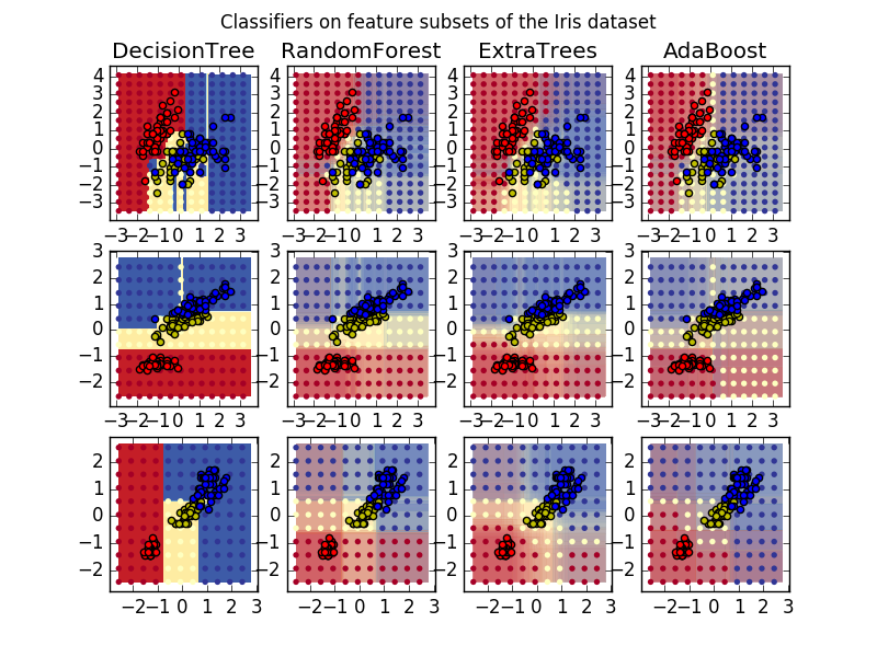
[Plot the determinants of a tree ensemble on an iris dataset](http://scikit-learn.org/0.18/auto_examples/ensemble/plot_forest_iris.html#sphx-glr-auto-examples-ensemble-plot-forest -iris-py)
-
Pixel importance in parallel forests of trees (http://scikit-learn.org/0.18/auto_examples/ensemble/plot_forest_importances_faces.html#sphx-glr-auto-examples-ensemble-plot-forest-importances -faces-py)
-
References
-
[B2001] Breiman, "Random Forest", Machine Learning, 45 (1), 5-32, 2001.
- [B1998] Breiman、 "Arcing Classifiers"、Annals of Statistics 1998
-
[GEW2006] P. Geurts, D. Ernst. , And L. Wehenkel, "Super Randomized Trees", Machine Learning, 63 (1), 3-42, 2006.
1.11.2.5. Evaluation of importance of features
The relative rank (ie, depth) of a feature used as a decision node in the tree can be used to assess the relative importance of that feature to the predictability of the target variable. The features used at the top of the tree contribute to the final predictive determination of the larger portion of the input sample. Therefore, * the expected proportion of samples they contribute to * can be used as an estimate of the relative importance * of the features (explanatory variables). By * averaging * these expected activity rates across several randomized trees, the * variance * of such estimates can be reduced * and used for feature selection. .. The following example is for each pixel of a face recognition task using the ExtraTreesClassifier model. Shows a color-coded representation of the relative reading.
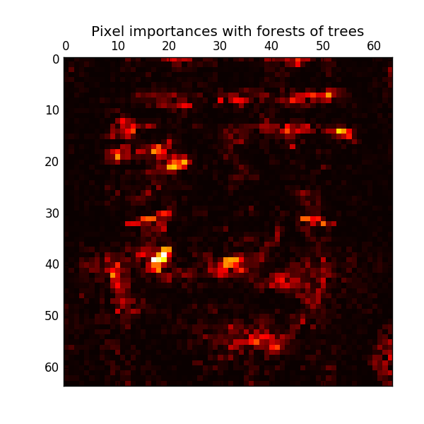
In practice, these estimates are stored in the fitted model as an attribute named feature_importances_. This is an array with positive values for the shape (n_features,) and a sum of 1.0. The higher the value, the more important the contribution of the match function to the predictive function.
- Example:
- Pixel importance in parallel forests of trees (http://scikit-learn.org/0.18/auto_examples/ensemble/plot_forest_importances_faces.html#sphx-glr-auto-examples-ensemble-plot-forest-importances -faces-py)
- Import features in the tree forest
1.11.2.6. Fully random tree embedding
RandomTreesEmbedding implements unsupervised data transformation. Using a completely random tree forest, RandomTreesEmbedding encodes the data by the index of the leaf where the data points end. This index is encoded in a K one-to-one way, leading to higher dimensional sparse binary coding. This coding is calculated very efficiently and can be used as the basis for other learning tasks. Code size and sparseness can be affected by choosing the number of trees and the maximum depth per tree. For each tree in the ensemble, the coding contains one entry. The maximum coding size is n_estimators * 2 ** max_depth, which is the maximum number of leaves in the forest.
The transformation performs an implicit nonparametric density estimation because adjacent data points are likely to be in the same leaf of the tree.
- Example:
- [Hash conversion using completely random tree](http://scikit-learn.org/0.18/auto_examples/ensemble/plot_random_forest_embedding.html#sphx-glr-auto-examples-ensemble-plot-random-forest-embedding -py)
- [Manifold learning of handwritten numbers: Local linear embedding, Isomap ...](http://scikit-learn.org/0.18/auto_examples/manifold/plot_lle_digits.html#sphx-glr-auto-examples-manifold-plot -lle-digits-py) compares nonlinear dimensionality reduction techniques for handwritten numbers.
- Feature transformation by tree ensemble Compares a supervised tree with an unmanaged tree-based feature transformation.
See also: Manifold Learning (http://scikit-learn.org/0.18/modules/manifold.html#manifold) The technique also helps to derive a non-linear representation of the feature space. These approaches also focus on dimensionality reduction.
1.11.3. AdaBoost
The module sklearn.ensemble is a common boosting algorithm introduced by Freund and Schapire in 1995. Includes AdaBoost [FS1995]. AdaBoost's core principle is to fit a sequence of weak learners (a model that is slightly better than a random guess, such as a small decision tree) to an iteratively modified version of the data. The predictions from all of them are combined by a weighted majority (or sum) to generate the final prediction. The data modification in each boosting iteration consists of applying weights $ w_1, w_2, ..., w_N $ to each of the training samples. Initially, all of these weights are set to $ w_i = 1 / N $, so the first step is to simply train the weak learner with the original data. At each iteration, the sample weights are changed individually and the training algorithm is reapplied to the reweighted data. In a given step, training examples that were incorrectly predicted by the boosted model evoked in the previous step will have an increased weight, and those that were correctly predicted will have a decreased weight. As the iterations progress, more and more difficult-to-predict cases are affected. Each subsequent weak learner is forced to focus on the examples missed by the weak learner before the sequence [HTF].
- AdaBoost can be used for both classification and regression problems.
- For multi-class classification, [AdaBoostClassifier](http://scikit-learn.org/0.18/modules/generated/sklearn.ensemble.AdaBoostClassifier.html#sklearn] which implements AdaBoost-SAMME and AdaBoost-SAMME.R [ZZRH2009] .ensemble.AdaBoostClassifier).
- For regression, use AdaBoostRegressor which implements AdaBoost.R2 [D1997].
1.11.3.1. Usage
The following example shows how to train with the AdaBoost classifier using 100 weak learners.
>>> from sklearn.datasets import load_iris
>>> from sklearn.ensemble import AdaBoostClassifier

>>> iris = load_iris()
>>> clf = AdaBoostClassifier(n_estimators=100)
>>> scores = cross_val_score(clf, iris.data, iris.target)
>>> scores.mean()
0.9...
The number of weak learners is controlled by the parameter n_estimators. The learning_rate parameter controls the weak learner's contribution to the final combination. By default, the weak learner is the Decision Stock (https://en.wikipedia.org/wiki/Decision_stump). You can specify a weak learner using the base_estimator parameter. The main parameters to adjust for good results are n_estimator and the complexity of the base estimator (for example, for a depth tree, the minimum required number of samples in depth max_depth or leaf min_samples_leaf). is.
-
Example:
-
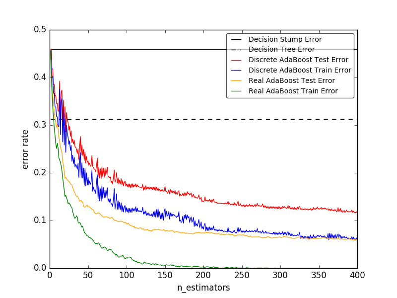
Discrete vs. real number AdaBoost Uses AdaBoost-SAMME and AdaBoost-SAMME.R to compare the classification errors of decision stumps, decision trees, and boosted decision stumps.
-
Multiclass AdaBoosted Decision Trees Shows the performance of AdaBoost-SAMME and AdaBoost-SAMME.R for multiclass problems.
-
2 classes of AdaBoost is AdaBoost- We use SAMME to show the decision boundary and decision function values for a two-class problem that is non-linearly separable.
-
Decision Tree Regression by AdaBoost is AdaBoost Shows regression by the .R2 algorithm.
-
References
-
[FS1995] Y. Freund and R. Schapire, "Deterministic Generalization of Online Learning and its Application to Boosting", 1997.
-
[ZZRH2009] J. Zhu, H.Zou, S.Rosset, T.Hastie. "Multiclass AdaBoost", 2009.
-
[D1997] Drucker. "Improvement of Regression Machine Using Boosting Technology", 1997.
-
[HTF] T. Hastie, R. Tibshirani and J. Friedman, "Elements of Statistical Learning Ed. 2", Springer, 2009.
1.11.4. Gradient Tree Boost
Gradient Tree Boost (https://en.wikipedia.org/wiki/Gradient_boosting) or Gradient Boost Regression Tree (GBRT) is a generalization that boosts to any differentiable loss function. GBRT is an accurate and effective off-the-shelf procedure that can be used for both regression and classification problems. The Gradient Tree Boosting model is used in a variety of areas, including web search rankings and ecology.
- The advantages of GBRT are:
- Natural treatment of mixed data (= heterogeneous features)
- Predictive power
- Robustness to outliers in output space (due to robust loss function)
- The disadvantages of GBRT are:
- Due to the sequential nature of boosting, it can hardly be parallelized.
The module sklearn.ensemble provides methods for both classification and regression with gradient boosted regression trees. Offers.
1.11.4.1. Classification
GradientBoostingClassifier supports both binary and multiclass classification. The following example shows how to fit a gradient boosting classifier as a weak learner with 100 determined strains.
>>> from sklearn.datasets import make_hastie_10_2
>>> from sklearn.ensemble import GradientBoostingClassifier

>>> X, y = make_hastie_10_2(random_state=0)
>>> X_train, X_test = X[:2000], X[2000:]
>>> y_train, y_test = y[:2000], y[2000:]

>>> clf = GradientBoostingClassifier(n_estimators=100, learning_rate=1.0,
...     max_depth=1, random_state=0).fit(X_train, y_train)
>>> clf.score(X_test, y_test)
0.913...
The number of weak learners (ie, regression trees) is controlled by the parameter n_estimators. Size of each tree sets the depth of the tree with max_depth ormax_leaf_nodes It can be controlled by setting the number of leaf nodes with. learning_rate is a hyperparameter of the range(0.0, 1.0]that controls overfitting by Shrinkage (http://scikit-learn.org/0.18/modules/ensemble.html#gradient-boosting-shrinkage). is.
** Note: ** A classification with two or more classes requires the induction of a n_classes regression tree at each iteration, so the total number of derived trees is equal to n_classes * n_estimators. For datasets with many classes, instead of GradientBoostingClassifier, [RandomForestClassifier] We strongly recommend that you use (http://scikit-learn.org/0.18/modules/generated/sklearn.ensemble.RandomForestClassifier.html#sklearn.ensemble.RandomForestClassifier).
1.11.4.2. Regression
GradientBoostingRegressor is a variety of regression losses that can be specified by the argument loss. Functions](http://scikit-learn.org/0.18/modules/ensemble.html#gradient-boosting-loss) is supported. The default loss function for regression is least squares ('ls').
>>> import numpy as np
>>> from sklearn.metrics import mean_squared_error
>>> from sklearn.datasets import make_friedman1
>>> from sklearn.ensemble import GradientBoostingRegressor

>>> X, y = make_friedman1(n_samples=1200, random_state=0, noise=1.0)
>>> X_train, X_test = X[:200], X[200:]
>>> y_train, y_test = y[:200], y[200:]
>>> est = GradientBoostingRegressor(n_estimators=100, learning_rate=0.1,
...     max_depth=1, random_state=0, loss='ls').fit(X_train, y_train)
>>> mean_squared_error(y_test, est.predict(X_test))
5.00...
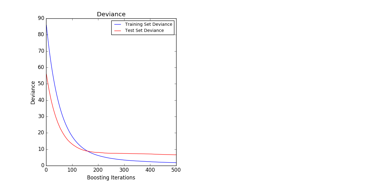
The figure below shows the Boston home price dataset (sklearn.datasets.load_boston). ) With minimal squared loss and a 500-based learner applied [GradientBoostingRegressor](http://scikit-learn.org/0.18/modules/generated/sklearn.ensemble.GradientBoostingRegressor.html#sklearn.ensemble. The result of GradientBoostingRegressor) is shown. The plot on the left shows the train and the test error at each iteration. The train error at each iteration is stored in the train_score_ attribute of the gradient boosting model. The test error at each iteration returns a generator that generates a prediction for each stage [staged_predict](http://scikit-learn.org/0.18/modules/generated/sklearn.ensemble.GradientBoostingRegressor.html#sklearn.ensemble. It can be obtained using the GradientBoostingRegressor.staged_predict) method. You can use such a plot to determine the optimal number of trees (n_estimators) by early stop. The plot on the right shows the feature imports that can be obtained using the feature_importances_ property.
1.11.4.3. Additional learning
GradientBoostingRegressor and GradientBoostingClassifier /modules/generated/sklearn.ensemble.GradientBoostingClassifier.html#sklearn.ensemble.GradientBoostingClassifier) both support warm_start = True. This allows you to add training to a model that you have already fitted.
>>> _ = est.set_params(n_estimators=200, warm_start=True)  # set warm_start and new nr of trees
>>> _ = est.fit(X_train, y_train) # fit additional 100 trees to est
>>> mean_squared_error(y_test, est.predict(X_test))
3.84...
1.11.4.4. Tree size control
The size of the regression tree-based learner defines the level of variable interaction captured by the gradient boosting model. In general, trees of depth h can capture interactions of degree h. There are two ways to control the size of individual regression trees.
Specifying max_depth = h completes a binary tree with a depth of h. Such a tree has (up to) a leaf node of 2 ** h and a partition node of 2 ** h-1.
Alternatively, you can use the max_leaf_nodes parameter to control the tree size by specifying the number of leaf nodes. In this case, the tree grows using the best-first search, where the node with the most improved impurities is expanded first. A tree with max_leaf_nodes = k has k-1 split nodes and can model interactions up to max_leaf_nodes-1.
We have found that max_leaf_nodes = k gives results comparable to max_depth = k-1, but training is much faster, but at the expense of slightly higher training errors. The max_leaf_nodes parameter corresponds to the variable J in the Gradient Boost chapter of [F2001] and is related to the ʻinteraction.depth parameter of the R's gbm package with max_leaf_nodes == interaction.depth + 1`.
1.11.4.5. Mathematical prescription
GBRT considers an additive model of the form:
F(x) = \sum_{m=1}^{M} \gamma_m h_m(x)
Where $ h_m (x) $ is a basis set, usually called a weak learner in the context of boosting. Gradient Tree Boosting uses a fixed size decision tree (http://scikit-learn.org/0.18/modules/tree.html#tree) as a weak learner. Decision trees have several capabilities that can be useful for boosting to enhance your ability to work with mixed data and model complex features. Like other boosting algorithms, GBRT builds the adder model in the forward phase.
F_m(x) = F_{m-1}(x) + \gamma_m h_m(x)
At each stage, the decision tree $ h_m (x) $ is the loss function $ L $ given the current model $ F_ {m-1} $ and its fit $ F_ {m-1} (x_i) $. Is selected to minimize.
F_m(x) = F_{m-1}(x) + \arg\min_{h} \sum_{i=1}^{n} L(y_i,
F_{m-1}(x_i) - h(x))
The initial model $ F_ {0} $ is problem-specific and usually chooses the mean of the target values for least squares regression.
Note: The initial model can also be specified with the init argument. The passed object must implement fit and prediction.
Gradient boost attempts to solve this minimization problem numerically through steepest descent. The steepest descent is the negative gradient of the loss function evaluated by the current model $ F_ {m-1} $, which can be calculated for any differentiable loss function.
F_m(x) = F_{m-1}(x) + \gamma_m \sum_{i=1}^{n} \nabla_F L(y_i,
F_{m-1}(x_i))
If you specify the line length and select the step length $ \ gamma_m $,
\gamma_m = \arg\min_{\gamma} \sum_{i=1}^{n} L(y_i, F_{m-1}(x_i)
- \gamma \frac{\partial L(y_i, F_{m-1}(x_i))}{\partial F_{m-1}(x_i)})
The algorithms for regression and classification differ only in the specific loss function used.
1.11.4.5.1. Loss function
The following loss functions are supported and can be specified using the parameter loss.
- Regression
- Least squares (
'ls'): Natural selection of regression due to good computational properties. The initial model is given by the average of the target values. - Minimum Absolute Deviation (
'lad'): Robustness function of regression. The initial model is given by the median of the target values. - Huber (
'huber'): Another robust robustness function that combines the least squares and the least absolute deviations. Use ʻalpha` to control sensitivity with respect to outliers (see [F2001] for details). - Quantile (
'quantile'): Loss function of quantile regression. Use0 <alpha <1to specify the quantile. You can use this loss function to create a predicted interval (Predicted Interval for Gradient Boost Regression) (http://scikit-learn.org/0.18/auto_examples/ensemble/plot_gradient_boosting_quantile.html#sphx-glr- (see auto-examples-ensemble-plot-gradient-boosting-quantile-py)). - Classification
- Binary classification (
'deviance'): Negative binomial log-likelihood loss function for binomial classification (provides probability estimation). The initial model is given by the log odds ratio. - Polynomial deviation (
'deviance'): Negative multinomial logarithm for multiclass classification with mutually exclusive classn_classes-likelihood loss function. It provides probability estimation. The initial model is given by the prior probabilities of each class. With each iteration, you need to build a regression tree that makes GBRT rather inefficient for datasets with many classes. - Exponential loss (
'exponential'): Same as AdaBoostClassifier Loss function. Examples of mislabeling than'deviance'are not very strong. Can only be used for binary classification.
1.11.4.6. Normalization
1.11.4.6.1. Shrinkage
[F2001] proposed a simple regularization strategy that scales the contribution of each weak learner by a factor. $ \ nu $:
F_m(x) = F_{m-1}(x) + \nu \gamma_m h_m(x)
The parameter $ \ nu $ is also called ** learning rate ** because it scales the step length of the gradient descent procedure. It can be set using the learning_rate parameter.
The parameter learning_rate interacts strongly with the parameter n_estimators, which matches the number of weak learners. The smaller the value of learning_rate, the more weak learners are needed to maintain constant training errors. Empirical evidence shows that smaller values for learning_rate improve test errors. [HTF2009] recommends setting the learning rate to a small constant (for example, learning_rate <= 0.1) and selecting n_estimators by early stop. For more information on the interaction of learning_rate and n_estimators, see [R2007].
1.11.4.6.2. Subsampling
[F1999] proposed a stochastic gradient descent that combines gradient boost with bootstrap average (bagging). At each iteration, the basic classifier is trained on the decimal subsample of the available training data. Subsamples are drawn without replacement. A typical value for subsample is 0.5.
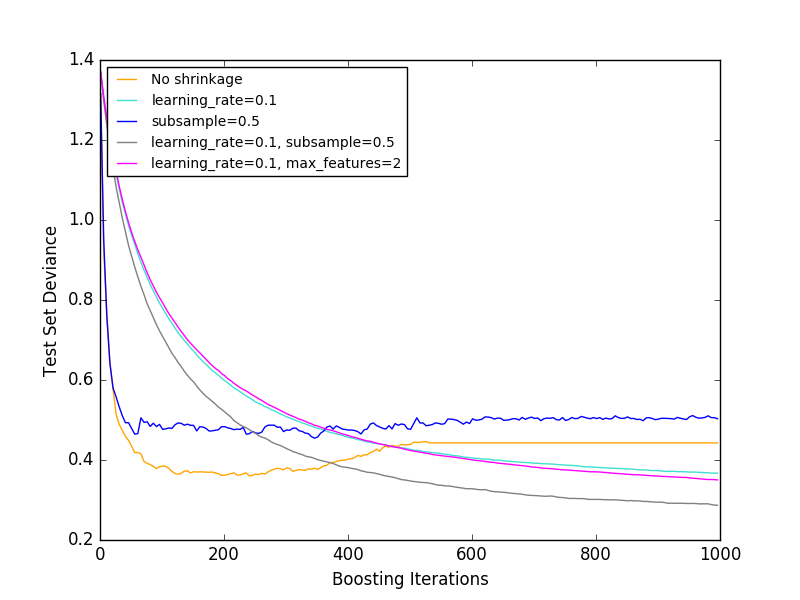
The figure below shows the effect of shrinkage and subsampling on the goodness of fit of the model. You can clearly see that the contraction does not contract. Subsampling with shrinkage can further improve the accuracy of the model. On the other hand, subsampling without shrinkage does not work very well.
Another strategy to reduce variance is similar to random splitting with RandomForestClassifier. It is to subsample the features. The number of subsampled features can be controlled by the max_features parameter.
Note: Decreasing the value of max_features can significantly reduce the runtime.
Stochastic gradient descent makes it possible to calculate out-of-bag estimates of test deviations by calculating the improvement in deviations for examples not included in the bootstrap sample (ie, out-of-bag examples). Improvements are stored in the attribute ʻoob_improvement_. ʻOob_improvement_ [i] retains the improvement in OOB sample loss when adding the i-th stage to the current forecast. Out-of-bag estimates can be used for model selection, such as determining the optimal number of iterations. OOB estimators are usually very pessimistic, so it is recommended that you use mutual validation instead and only use OOB if mutual validation takes too long.
- Example:
- Gradient Boosting Regularization
- Gradient Boost Out of Bag Estimate
- Random Forest OOB Error
1.11.4.7. Interpretation
Individual decision trees can be easily interpreted by simply visualizing the tree structure. However, the gradient boosting model contains hundreds of regression trees and cannot be easily interpreted by visual inspection of individual trees. Fortunately, many techniques have been proposed for summarizing and interpreting gradient boosting models.
1.11.4.7.1. Importance of features
In many cases, features do not evenly contribute to predicting the target response. In many cases, most of the features are actually irrelevant. When interpreting the model, the first question is usually what are their important features and how they contribute to predicting the target response.
The individual decision trees essentially perform feature selection by selecting the appropriate division points. This information can be used to measure the importance of each feature. The basic idea is that the more often a feature is used at a tree split point, the more important it becomes. This important concept can be extended to a decision tree ensemble by simply averaging the feature importance of each tree (for more information, see Importance Rating (http: // scikit-). See learn.org/0.18/modules/ensemble.html#random-forest-feature-importance).
The feature importance score of the fit gradient boosting model can be accessed from the feature_importances_ property.
>>> from sklearn.datasets import make_hastie_10_2
>>> from sklearn.ensemble import GradientBoostingClassifier

>>> X, y = make_hastie_10_2(random_state=0)
>>> clf = GradientBoostingClassifier(n_estimators=100, learning_rate=1.0,
...     max_depth=1, random_state=0).fit(X, y)
>>> clf.feature_importances_
array([ 0.11,  0.1 ,  0.11,  ...
- Example:
- Gradient Boost Regression
1.11.4.7.2. Partially dependent
The partial dependency plot (PDP) shows the dependency between the target response and a set of "target" features that margin the values of all other features ("complementary" features). Intuitively, we can interpret partial dependence as a function of "target" features [2] and as an expected target response [1]. Due to the limits of human perception, the size of the target feature set must be small (usually one or two), so the target feature is usually selected from among the most important features. The figure below shows four unidirectional and unidirectional partially dependent plots of a California residential dataset.
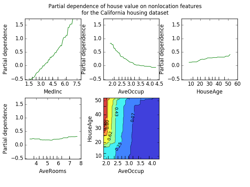
One-way PDP teaches the interaction between target response and target features (eg, linear, non-linear). The plot in the upper left of the figure above shows the effect of average income within a district on median home prices. We can clearly see the linear relationship between them.
A PDP with two target features-shows an interaction between the two features. For example, the two-variable PDP in the figure above shows how the median home price depends on the joint value of household age and average. Number of occupants per household. You can clearly see the interaction between the two features. For two or more people, the price of the house is almost independent of the age of the house, while for less than two people it is strongly age-dependent.
The module partial_dependence is a convenient function plot_partial_dependence that creates unidirectional and bidirectional partial dependency plots. sklearn.ensemble.partial_dependence.plot_partial_dependence). The following example shows how to create a grid of partially dependent graphs. Two unidirectional PDPs with features 0 and 1 and bidirectional PDPs between the two features.
>>> from sklearn.datasets import make_hastie_10_2
>>> from sklearn.ensemble import GradientBoostingClassifier
>>> from sklearn.ensemble.partial_dependence import plot_partial_dependence

>>> X, y = make_hastie_10_2(random_state=0)
>>> clf = GradientBoostingClassifier(n_estimators=100, learning_rate=1.0,
...     max_depth=1, random_state=0).fit(X, y)
>>> features = [0, 1, (0, 1)]
>>> fig, axs = plot_partial_dependence(clf, X, features)
For multiclass models, you must use the label argument to set the class label that creates the PDP.
>>>
>>> from sklearn.datasets import load_iris
>>> iris = load_iris()
>>> mc_clf = GradientBoostingClassifier(n_estimators=10,
...     max_depth=1).fit(iris.data, iris.target)
>>> features = [3, 2, (3, 2)]
>>> fig, axs = plot_partial_dependence(mc_clf, X, features, label=0)
If you want the raw value of a partially dependent function instead of a plot, then [partial_dependence](http://scikit-learn.org/0.18/modules/generated/sklearn.ensemble.partial_dependence.partial_dependence.html#sklearn.ensemble. You can use the partial_dependence.partial_dependence) function:
>>>
>>> from sklearn.ensemble.partial_dependence import partial_dependence

>>> pdp, axes = partial_dependence(clf, [0], X=X)
>>> pdp
array([[ 2.46643157,  2.46643157, ...
>>> axes
[array([-1.62497054, -1.59201391, ...
The function requires either the argument grid, which specifies the value of the target feature for which the partial dependency function should be evaluated, or the argument X, which is a simple mode for automatically creating a grid from training data. To do. If X is specified, the axis value returned by the function will be the axis for each target feature.
For each value of the "target" feature in grid, the partially dependent function needs to estrange the prediction of the tree over all possible values of the" complementary "feature. In decision trees, this feature can be evaluated efficiently without reference to training data. Weighted tree traversal is performed for each gridpoint: if the split node contains "target" features, it branches to the corresponding left or right. Otherwise, follow both branches. Each branch is weighted with the percentage of training samples in that branch. Finally, the partial dependency is given by the weighted average of all the reefs visited. For tree ensembles, the results for individual trees are averaged again.
-
Footnote
-
[1] In the loss ='deviation'classification, the target response is logit (p).
-
[2] More precisely, the expectation of the target response after considering the initial model. The partial dependency graph does not include the init model.
-
Example:
-
References
-
[F2001](1, 2, 3) J. Friedman, "Greedy Function Approximation: Gradient Boost Machine", Annual Statistical Report, Vol. Volume 29, Issue 5, 2001.
-
[F1999] Friedman, "Stochastic Gradient Boost", 1999
-
[HTF2009] Hastie, R. Tibshirani and J. Friedman, "Elements of Statistical Learning Ed. 2", Springer, 2009.
-
[R2007] Ridgeway, "Generalized Boosted Models: gbm Package Guide", 2007
1.11.5. VotingClassifier
The idea behind the voting classifier implementation is to combine conceptually different machine learning classifiers and predict class labels using majority voting or average predictive probability (soft voting). Such a classifier can be useful in a set of models that also work well to balance individual weaknesses.
1.11.5.1. Labels for the majority of classes (majority / careful selection)
In a majority vote, the predicted class label for a particular sample is the class label that represents the majority (mode) of the class label predicted by the individual classifiers.
For example, the prediction of a given sample
- Classifier 1 → Class 1
- Classifier 2 → Class 1
- Classifier 3 → Class 2
VotingClassifier (voting ='hard') classifies samples as "class 1" based on a large number of class labels.
For equivalence, VotingClassifier selects classes based on ascending sort order. For example, in the following scenario
- Classifier 1 → Class 2
- Classifier 2 → Class 1
Class label 1 is assigned to the sample.
1.11.5.1.1. Usage
The following example shows how to fit a majority rule classifier.
>>> from sklearn import datasets
>>> from sklearn.model_selection import cross_val_score
>>> from sklearn.linear_model import LogisticRegression
>>> from sklearn.naive_bayes import GaussianNB
>>> from sklearn.ensemble import RandomForestClassifier
>>> from sklearn.ensemble import VotingClassifier

>>> iris = datasets.load_iris()
>>> X, y = iris.data[:, 1:3], iris.target

>>> clf1 = LogisticRegression(random_state=1)
>>> clf2 = RandomForestClassifier(random_state=1)
>>> clf3 = GaussianNB()

>>> eclf = VotingClassifier(estimators=[('lr', clf1), ('rf', clf2), ('gnb', clf3)], voting='hard')

>>> for clf, label in zip([clf1, clf2, clf3, eclf], ['Logistic Regression', 'Random Forest', 'naive Bayes', 'Ensemble']):
...     scores = cross_val_score(clf, X, y, cv=5, scoring='accuracy')
...     print("Accuracy: %0.2f (+/- %0.2f) [%s]" % (scores.mean(), scores.std(), label))
Accuracy: 0.90 (+/- 0.05) [Logistic Regression]
Accuracy: 0.93 (+/- 0.05) [Random Forest]
Accuracy: 0.91 (+/- 0.04) [naive Bayes]
Accuracy: 0.95 (+/- 0.05) [Ensemble]
1.11.5.2. Weighted average probability (soft voting)
In contrast to the majority of votes (hard votes), soft votes return the class label as the total predicted probability argmax.
Specific weights can be assigned to each classifier via the weights parameter. Given the weights, the predicted class probabilities for each classifier are collected, the classifier weights are multiplied, and averaged. The last class label is derived from the class label with the highest average probability.
To explain this with a simple example, suppose there are three classifiers, w1 = 1, w2 = 1, and w3 = 1, and three classes of classification problems that assign equal weights to all classifiers. I will.
The weighted average probability of the sample is calculated as follows:
| Classifier | Class 1 | Class 2 | Class 3 |
|---|---|---|---|
| Classifier 1 | w1 * 0.2 | w1 * 0.5 | w1 * 0.3 |
| Classification machine 2 | w2 * 0.6 | w2 * 0.3 | w2 * 0.1 |
| Classifier 3 | w3 * 0.3 | w3 * 0.4 | w3 * 0.3 |
| weighted average | 0.37 | 0.4 | 0.23 |
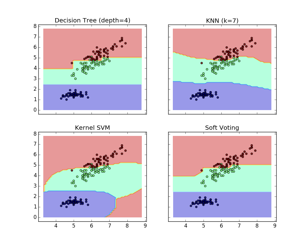
Here, the predictive class label is 2 because it has the highest average probability. The following example shows how the decision area changes when the soft VotingClassifier is used based on a linear support vector machine, a decision tree, and a K-nearest neighbor classifier.
>>> from sklearn import datasets
>>> from sklearn.tree import DecisionTreeClassifier
>>> from sklearn.neighbors import KNeighborsClassifier
>>> from sklearn.svm import SVC
>>> from itertools import product
>>> from sklearn.ensemble import VotingClassifier

>>> # Loading some example data
>>> iris = datasets.load_iris()
>>> X = iris.data[:, [0,2]]
>>> y = iris.target

>>> # Training classifiers
>>> clf1 = DecisionTreeClassifier(max_depth=4)
>>> clf2 = KNeighborsClassifier(n_neighbors=7)
>>> clf3 = SVC(kernel='rbf', probability=True)
>>> eclf = VotingClassifier(estimators=[('dt', clf1), ('knn', clf2), ('svc', clf3)], voting='soft', weights=[2,1,2])

>>> clf1 = clf1.fit(X,y)
>>> clf2 = clf2.fit(X,y)
>>> clf3 = clf3.fit(X,y)
>>> eclf = eclf.fit(X,y)
1.11.5.3. Using Voting Classifier with Grid Search
VotingClassifier can also be used with GridSearch to adjust the hyperparameters of individual estimators.
>>> from sklearn.model_selection import GridSearchCV
>>> clf1 = LogisticRegression(random_state=1)
>>> clf2 = RandomForestClassifier(random_state=1)
>>> clf3 = GaussianNB()
>>> eclf = VotingClassifier(estimators=[('lr', clf1), ('rf', clf2), ('gnb', clf3)], voting='soft')

>>> params = {'lr__C': [1.0, 100.0], 'rf__n_estimators': [20, 200],}

>>> grid = GridSearchCV(estimator=eclf, param_grid=params, cv=5)
>>> grid = grid.fit(iris.data, iris.target)
1.11.5.3.1 Usage
To predict class labels based on predicted class probabilities (VotingClassifier scikit-lear estimators must support the predict_proba method)
>>> eclf = VotingClassifier(estimators=[('lr', clf1), ('rf', clf2), ('gnb', clf3)], voting='soft')
You can optionally weight individual classifiers.
>>> eclf = VotingClassifier(estimators=[('lr', clf1), ('rf', clf2), ('gnb', clf3)], voting='soft', weights=[2,5,1])
[scikit-learn 0.18 User Guide 1. Supervised Learning](http://qiita.com/nazoking@github/items/267f2371757516f8c168#1-%E6%95%99%E5%B8%AB%E4%BB%98 From% E3% 81% 8D% E5% AD% A6% E7% BF% 92)
© 2010 --2016, scikit-learn developers (BSD license).