[PYTHON] [Translation] scikit-learn 0.18 User Guide 3.3. Model evaluation: Quantify the quality of prediction
Google translated http://scikit-learn.org/0.18/modules/model_evaluation.html [scikit-learn 0.18 User Guide 3. Model Selection and Evaluation](http://qiita.com/nazoking@github/items/267f2371757516f8c168#3-%E3%83%A2%E3%83%87%E3%83] From% AB% E3% 81% AE% E9% 81% B8% E6% 8A% 9E% E3% 81% A8% E8% A9% 95% E4% BE% A1)
3.3. Model Evaluation: Quantify the quality of predictions
There are three different approaches to assessing the quality of model predictions.
-** Estimator Score Method : The estimator has a score method that provides default metrics for problems designed to be resolved. This is not on this page, but in the documentation for each estimator.
- Scoring parameters : Model evaluation tool (model_selection.cross_val_score) using Cross validation .org / 0.18 / modules / generated / sklearn.model_selection.cross_val_score.html # sklearn.model_selection.cross_val_score) and [model_selection.GridSearchCV](http://scikit-learn.org/0.18/modules/generated/sklearn.model_selection. GridSearchCV.html # sklearn.model_selection.GridSearchCV), etc.) relies on an internal scoring strategy. For this, see Scoring Parameters: Definition of Model Evaluation Rules (# 331-% E5% BE% 97% E7% 82% B9% E3% 83% 91% E3% 83% A9% E3% 83% A1% E3% 83% BC% E3% 82% BF% E3% 83% A2% E3% 83% 87% E3% 83% AB% E8% A9% 95% E4% BE% A1% E3% 83% AB% E3% It is explained in the section 83% BC% E3% 83% AB% E3% 81% AE% E5% AE% 9A% E7% BE% A9).
- Metric function **: The metric module implements a function that evaluates prediction errors for a specific purpose. These metrics are described in detail in the sections on classification metrics, multi-label ranking metrics, regression metrics, and clustering metrics.
Finally, dummy evaluators are useful for getting baseline values for those metrics for random prediction.
-** See: ** For "pair-by-pair" metrics, differences between samples and estimates or predictions, see Pairwise Metrics, Affinity and Kernels (http://scikit-learn.org/0.18/modules). See the section at /metrics.html#metrics).
3.3.1. Scoring parameters: Definition of model evaluation rules
model_selection.GridSearchCV and model_selection.cross_val_score Model selection and evaluation using tools such as .org / 0.18 / modules / generated / sklearn.model_selection.cross_val_score.html # sklearn.model_selection.cross_val_score) has a scoring parameter that controls the metrics applied to the metrics. To use.
3.3.1.1. General case: Predefined value
For the most common use cases, you can use the scoring parameter to specify a scoring object. The table below shows all possible values. All scorer objects follow the rule that ** higher return values are better than lower return values **. Therefore, the distance between the model and the data, such as metrics.mean_squared_error The metric you measure is available as neg_mean_squared_error, which returns the negative value of the metric.
| Scoring | Function | Comment |
|---|---|---|
| Classification | ||
| ‘accuracy’ | metrics.accuracy_score |
|
| ‘average_precision’ | metrics.average_precision_score |
|
| ‘f1’ | metrics.f1_score |
For binary targets |
| ‘f1_micro’ | metrics.f1_score |
Micro averaging |
| ‘f1_macro’ | metrics.f1_score |
Macro averaging |
| ‘f1_weighted’ | metrics.f1_score |
weighted average |
| ‘f1_samples’ | metrics.f1_score |
Multi-label sample |
| ‘neg_log_loss’ | metrics.log_loss |
predict_probaNeed support |
| ‘precision’ etc. | metrics.precision_score |
The suffix is'f1'It applies in the same way as. |
| ‘recall’ etc. | metrics.recall_score |
The suffix is'f1'It applies in the same way as. |
| ‘roc_auc’ | metrics.roc_auc_score |
|
| Clustering | ||
| ‘adjusted_rand_score’ | metrics.adjusted_rand_score |
|
| Regression | ||
| ‘neg_mean_absolute_error’ | metrics.mean_absolute_error |
|
| ‘neg_mean_squared_error’ | metrics.mean_squared_error |
|
| ‘neg_median_absolute_error’ | metrics.median_absolute_error |
|
| ‘r2’ | metrics.r2_score |
Usage examples:
>>>
>>> from sklearn import svm, datasets
>>> from sklearn.model_selection import cross_val_score
>>> iris = datasets.load_iris()
>>> X, y = iris.data, iris.target
>>> clf = svm.SVC(probability=True, random_state=0)
>>> cross_val_score(clf, X, y, scoring='neg_log_loss')
array([-0.07..., -0.16..., -0.06...])
>>> model = svm.SVC()
>>> cross_val_score(model, X, y, scoring='wrong_choice')
Traceback (most recent call last):
ValueError: 'wrong_choice' is not a valid scoring value. Valid options are ['accuracy', 'adjusted_rand_score', 'average_precision', 'f1', 'f1_macro', 'f1_micro', 'f1_samples', 'f1_weighted', 'neg_log_loss', 'neg_mean_absolute_error', 'neg_mean_squared_error', 'neg_median_absolute_error', 'precision', 'precision_macro', 'precision_micro', 'precision_samples', 'precision_weighted', 'r2', 'recall', 'recall_macro', 'recall_micro', 'recall_samples', 'recall_weighted', 'roc_auc']
-** Note: ** The values listed by the ValueError exception correspond to the functions that measure predictive accuracy described in the next section. The scorer objects for these functions are stored in the dictionary sklearn.metrics.SCORERS.
3.3.1.2. Define a scoring strategy from a metric function
The module sklearn.metric also exposes a set of simple functions that measure measured values and forecast errors given a forecast:
--Functions ending in _score return the value to maximize.
--Functions ending in _error or _loss return a value to return to the minimum value. When converting to a scorer object using make_scorer, the greater_is_better parameter Is set to False (True by default, see parameter description below).
The metrics that can be used in various machine learning tasks are described in detail in the sections below.
Many metrics may require additional parameters such as fbeta_score. Therefore, there is no name to use as the scoring value. In such cases, you need to generate an appropriate scoring object. The easiest way to generate a callable object is to use make_scorer. The way. This function transforms the metric into a callable object that can be used for model evaluation.
One typical use case is to wrap an existing metric function from the library with a non-default value for the parameter, such as the beta parameter of the fbeta_score function.
>>> from sklearn.metrics import fbeta_score, make_scorer
>>> ftwo_scorer = make_scorer(fbeta_score, beta=2)
>>> from sklearn.model_selection import GridSearchCV
>>> from sklearn.svm import LinearSVC
>>> grid = GridSearchCV(LinearSVC(), param_grid={'C': [1, 10]}, scoring=ftwo_scorer)
The second use case is to build a completely custom scorer object from a simple python function using make_scorer which can take some parameters:
--Python function to use (my_custom_loss_func in the example below)
--Whether the python function returns a score (default greater_is_better = True) or loss (greater_is_better = False). In case of loss, the scorer object invalidates the output of the python function and the scorer returns a higher value for a better model.
--Classification metrics only: Whether the Python function you provided requires continuous decision certainty (needs_threshold = True) The default value is False.
--Additional parameters such as beta and labels for f1_score.
The following example creates a custom scorer and uses the greater_is_better parameter.
>>> import numpy as np
>>> def my_custom_loss_func(ground_truth, predictions):
...     diff = np.abs(ground_truth - predictions).max()
...     return np.log(1 + diff)
...
>>> # loss_func is my_custom_loss_Disables the return value of func.
>>> #This is the ground_np if there is a value of truth and the prediction defined below.log(2)、0.It will be 693.
>>> loss  = make_scorer(my_custom_loss_func, greater_is_better=False)
>>> score = make_scorer(my_custom_loss_func, greater_is_better=True)
>>> ground_truth = [[1, 1]]
>>> predictions  = [0, 1]
>>> from sklearn.dummy import DummyClassifier
>>> clf = DummyClassifier(strategy='most_frequent', random_state=0)
>>> clf = clf.fit(ground_truth, predictions)
>>> loss(clf,ground_truth, predictions)
-0.69...
>>> score(clf,ground_truth, predictions)
0.69...
3.3.1.3. Implementation of original scoring object
You can generate a more flexible model scorer by building your own scoring object from scratch without using the make_scorer factory. In order for the callable object to be a scorer, it must meet the protocol specified by the following two rules.
--Can be called with (estimator, X, y). ʻEstimator is the model to evaluate, Xis the validation data, andy is the measured target of X(with supervised) orNone(without supervised). --Refer toy and return a floating point number that quantifies the ʻestimator predicted quality on X. Again, the higher the number, the better, by convention, so if the scorer returns a loss, you should invalidate that value.
3.3.2. Classification metric
sklearn.metrics Module implements several loss, score, and utility functions to measure classification performance To do. Some metrics may require probability estimation of positive classes, confidence values, or binary decisions. In most implementations, the sample_weight parameter can be used to allow each sample to make a weighted contribution to the overall score.
These are limited to binary classification:
| matthews_corrcoef(y_true、y_pred [、...]) | Binary class Matthews correlation coefficient(MCC) |
| precision_recall_curve(y_true、probas_pred) | Adaptation rate for various probability thresholds-Calculate recall pairs |
| roc_curve(y_true、y_score [、pos_label、...]) | Operating characteristics of the receiver(ROC) |
These also work in multi-class:
| cohen_kappa_score(y1、y2 [、labels、weights]) | Cohen's kappa: Statistics that measure agreements between annotators. |
| confusion_matrix(y_true、y_pred [、labels、...]) | Calculate the confusion matrix to evaluate the accuracy of the classification |
| hinge_loss(y_true、pred_decision [、labels、...]) | Average hinge loss(Denormalized) |
These also work for multi-labels:
| accuracy_score(y_true、y_pred [、normalize、...]) | Accuracy classification score. |
| classification_report(y_true、y_pred [、...]) | Create a text report showing key classification metrics |
| f1_score(y_true、y_pred [、labels、...]) | Calculate the F1 score. This is also called balanced F score or F major |
| fbeta_score(y_true、y_pred、beta [、labels、...]) | Calculate F Beta Score |
| hamming_loss(y_true、y_pred [、labels、...]) | Calculate the average humming loss. |
| jaccard_similarity_score(y_true、y_pred [、...]) | Jaccard similarity score |
| log_loss(y_true、y_pred [、eps、normalize、...]) | Log loss, also known as logistic loss or cross entropy loss. |
| precision_recall_fscore_support(y_true、y_pred) | Conformity rate, recall rate, F of each class-Calculate measure and support |
| precision_score(y_true、y_pred [、labels、...]) | Calculate the precision |
| recall_score(y_true、y_pred [、labels、...]) | Calculate recall |
| zero_one_loss(y_true、y_pred [、normalize、...]) | Zero classification loss. |
These work in binary and multi-label (not multi-class)
| average_precision_score(y_true、y_score [、...]) | Average accuracy from predicted score(AP) |
| roc_auc_score(y_true、y_score [、average、...]) | Area under the curve from the predicted score(AUC) |
The following subsections describe each of these functions and pre-empt some notes on defining common APIs and metrics.
3.3.2.1. From binary to multi-class and multi-label
Basically, some metrics are defined for the binary classification task ([f1_score](http://scikit-learn.org/0.18/modules/generated/sklearn.metrics.f1_score.html#sklearn. metrics.f1_score), roc_auc_score. In such cases, by default only the positive label is evaluated and the positive class is labeled 1 (although it can be configured with the pos_label parameter).
When you extend a binary metric to a multi-class or multi-label problem, the data is treated as a collection of binary problems (one for each class). There are several ways to average binary metric calculations across a set of classes, which is useful in some scenarios. If possible, you should choose between these using the ʻaverage` parameter.
--" macro " calculates the average of binary metrics and gives equal weights to each class. Nevertheless, for problems where infrequent classes are important, macro averaging can be a way to emphasize performance. On the other hand, the assumption that all classes are equally important is often not true, so macro averaging overemphasizes poor performance in rare classes in general.
--" weighted " Class imbalances are "weighted" by calculating the average of binary metrics weighted by the existence of each class's score in a true data sample.
-"micro" contributes equally to the overall metric for each sample class pair (except for sample weight results). Instead of summing the per-class metrics, sum the dividends and divisors that make up the per-class metrics to calculate the overall quotient. Microaveraging may take precedence in multi-label settings, including multi-class classifications that ignore a large number of classes.
-"samples" applies only to multi-label problems. Instead, it calculates the metric for the true and predicted classes of each sample of the merit data and returns its (sample_weight --weighted) average.
--Selecting ʻaverage = None` returns an array containing the scores for each class.
Multi-class data is provided as an array of class labels metrically like a binary target, while multi-label data is cell [i, j" if sample ʻi has label j. ] `Returns the value 1 otherwise.
3.3.2.2. Accuracy score
accuracy_score The function is an accurate predictive percentage (default) or count (normalize). = False) is calculated.
For multi-label classification, this function returns a subset of precision. If the entire set of predicted labels in the sample exactly matches the actual set of labels, the subset precision is 1.0. Otherwise it is 0.0.
\texttt{accuracy}(y, \hat{y}) = \frac{1}{n_\text{samples}} \sum_{i=0}^{n_\text{samples}-1} 1(\hat{y}_i = y_i)
Where $ 1 (x) $ is the Indicator Function (https://en.wikipedia.org/wiki/Indicator_function).
>>> import numpy as np
>>> from sklearn.metrics import accuracy_score
>>> y_pred = [0, 2, 1, 3]
>>> y_true = [0, 1, 2, 3]
>>> accuracy_score(y_true, y_pred)
0.5
>>> accuracy_score(y_true, y_pred, normalize=False)
2
For multi-label with binary label indicator:
>>> accuracy_score(np.array([[0, 1], [1, 1]]), np.ones((2, 2)))
0.5
--Example: --Testing the Importance of Classification Scores in Permutations in an Example of Using Precision Scores Using Dataset Permutations (http://scikit-learn.org/0.18/auto_examples/feature_selection/plot_permutation_test_for_classification.html#sphx-glr See (-auto-examples-feature-selection-plot-permutation-test-for-classification-py).
3.3.2.3. Kappa coefficient
The function cohen_kappa_score is the [Kappa coefficient](https://en.wikipedia. org / wiki / Cohen% 27s_kappa) is calculated. This scale is intended to compare labeling by different human annotators. The κ score (see docstring) is a number between -1 and 1. Scores above 8 are generally considered good matches. Below zero means no agreement (virtually random label). The κ score can be calculated for binary or multi-class questions, but not for multi-label questions (unless you manually calculate the score for each label) and for two or more annotations.
>>> from sklearn.metrics import cohen_kappa_score
>>> y_true = [2, 0, 2, 2, 0, 1]
>>> y_pred = [0, 0, 2, 2, 0, 2]
>>> cohen_kappa_score(y_true, y_pred)
0.4285714285714286
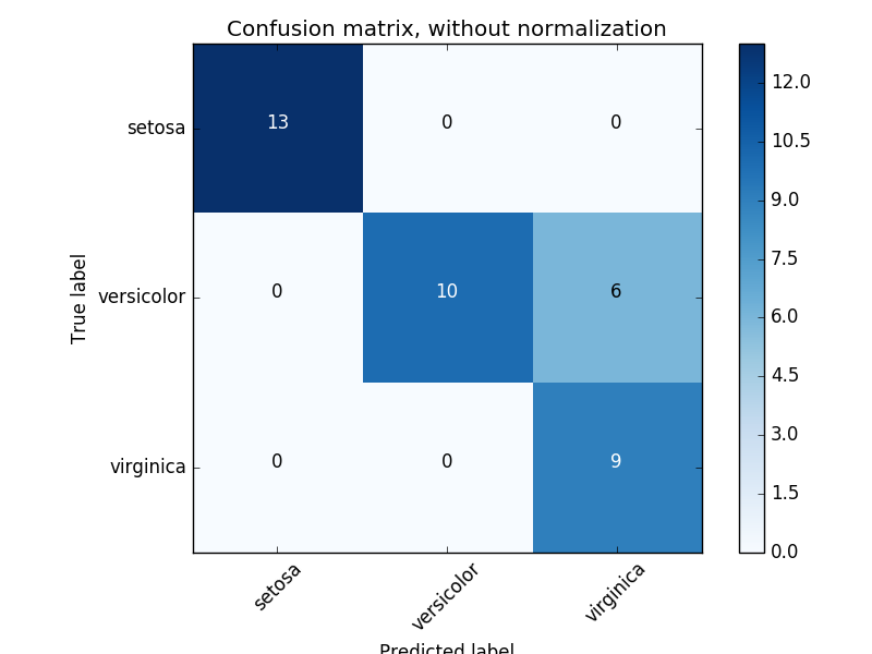
3.3.2.4. Confusion matrix
The confusion_matrix function is the Confusion Matrix (https://en.wikipedia. Evaluate classification accuracy by calculating (org / wiki / Confusion_matrix). By definition, the confusion matrix entries $ i, j $ are the actual observations of group $ i $, but are expected to belong to group $ j $. Here is an example:
>>> from sklearn.metrics import confusion_matrix
>>> y_true = [2, 0, 2, 2, 0, 1]
>>> y_pred = [0, 0, 2, 2, 0, 2]
>>> confusion_matrix(y_true, y_pred)
array([[2, 0, 0],
       [0, 0, 1],
       [1, 0, 2]])
A visual representation of such a confusion matrix (this figure is the Confusion Matrix (http://scikit-learn.org/0.18/auto_examples/model_selection/plot_confusion_matrix.html#sphx-glr-auto-examples-). An example of model-selection-plot-confusion-matrix-py)).
For binary problems, you can get true negative, false positive, false negative and true positive counts as follows:
--Example: --For an example of using a confusion matrix to evaluate the output quality of a classifier, see "[Confusion Matrix](http://scikit-learn.org/0.18/auto_examples/model_selection/plot_confusion_matrix.html#sphx-glr-auto". -examples-model-selection-plot-confusion-matrix-py) ". --For an example of using a confusion matrix to classify handwritten numbers, see Handwritten Number Recognition (http://scikit-learn.org/0.18/auto_examples/classification/plot_digits_classification.html#sphx-glr-auto- See examples-classification-plot-digits-classification-py). --For an example of classifying text documents using the confusion matrix, see [Classifying Text Documents Using Sparse Functions](http://scikit-learn.org/0.18/auto_examples/text/document_classification_20newsgroups.html#sphx- glr-auto-examples-text-document-classification-20newsgroups-py).
3.3.2.5. Classification report
The classification_report function creates a text report showing the major classification metrics. The following is a small example of a custom target_names and an estimated label.
>>> from sklearn.metrics import classification_report
>>> y_true = [0, 1, 2, 2, 0]
>>> y_pred = [0, 0, 2, 1, 0]
>>> target_names = ['class 0', 'class 1', 'class 2']
>>> print(classification_report(y_true, y_pred, target_names=target_names))
             precision    recall  f1-score   support

    class 0       0.67      1.00      0.80         2
    class 1       0.00      0.00      0.00         1
    class 2       1.00      0.50      0.67         2

avg / total       0.67      0.60      0.59         5
--Example: --For an example of using the Handwritten Number Classification Report, see Handwritten Number Recognition (http://scikit-learn.org/0.18/auto_examples/classification/plot_digits_classification.html#sphx-glr-auto-examples-classification-plot) See -digits-classification-py). --For an example of using a text document classification report, see "Classifying text documents using sparse functions" (http://scikit-learn.org/0.18/auto_examples/text/document_classification_20newsgroups.html#sphx-glr-auto- See examples-text-document-classification-20newsgroups-py). --For an example of using a grid search classification report with nested mutual validation, see Parameter Estimating Using Grid Search with Mutual Validation (http://scikit-learn.org/0.18/auto_examples/model_selection/grid_search_digits.html). See # sphx-glr-auto-examples-model-selection-grid-search-digits-py).
3.3.2.6. Humming loss
hamming_loss calculates the average humming loss or humming distance between two sets of samples. To do. If $ \ hat {y} j $ is the predicted value for the $ j $ th label of the given sample, then $ y_j $ is the corresponding true value and $ n \ text {labels} $ is the class or The number of labels, the humming loss $ L_ {Hamming} $, is defined as follows.
L_{Hamming}(y, \hat{y}) = \frac{1}{n_\text{labels}} \sum_{j=0}^{n_\text{labels} - 1} 1(\hat{y}_j \not= y_j)
Where $ 1 (x) $ is the Indicator Function (https://en.wikipedia.org/wiki/Indicator_function).
>>> from sklearn.metrics import hamming_loss
>>> y_pred = [1, 2, 3, 4]
>>> y_true = [2, 2, 3, 4]
>>> hamming_loss(y_true, y_pred)
0.25
For multi-label with binary label indicator:
>>>
>>> hamming_loss(np.array([[0, 1], [1, 1]]), np.zeros((2, 2)))
0.75
** (Note) ** In the multi-class classification, the Hamming loss is [Zero One Loss](# 33213-% E3% 82% BC% E3% 83% AD1% E3% 81% A4% E3% 81% AE% E6. % 90% 8D% E5% A4% B1) Corresponds to the Hamming distance between y_true and y_pred, which is similar to a function. However, one-to-one losses penalize predictive sets that do not exactly match the true set, while humming losses penalize individual labels. Therefore, the humming loss capped by the loss of zero 1 is always between 0 and 1, and predicting the proper subset or superset of the true label is humming between zero and 1. The loss will be eliminated.
3.3.2.7. Jacquard Similarity Coefficient Score
jaccard_similarity_score The function is also called the Jaccard index between paired label sets [Jaccard-like] Calculates the average (default) or sum of Gender Factors (https://en.wikipedia.org/wiki/Jaccard_index). The Jaccard similarity coefficient for the $ i $ th sample with the measured label set $ y_i $ and the predicted label set $ \ hat {y} _i $ is defined as follows:
J(y_i, \hat{y}_i) = \frac{|y_i \cap \hat{y}_i|}{|y_i \cup \hat{y}_i|}.
For binary and multiclass classification, the Jaccard similarity coefficient score is equal to the classification accuracy.
>>> import numpy as np
>>> from sklearn.metrics import jaccard_similarity_score
>>> y_pred = [0, 2, 1, 3]
>>> y_true = [0, 1, 2, 3]
>>> jaccard_similarity_score(y_true, y_pred)
0.5
>>> jaccard_similarity_score(y_true, y_pred, normalize=False)
2
For multi-label with binary label indicator:
>>>
>>> jaccard_similarity_score(np.array([[0, 1], [1, 1]]), np.ones((2, 2)))
0.75
3.3.2.8. Accuracy, recall, F-measure
Intuitively, the precision rate (https://en.wikipedia.org/wiki/Precision_and_recall#Precision) is the ability of the classifier to prevent negative samples from being labeled as positive, and reproduced. Rate is the ability of the classifier to find all positive samples. The F-values ($ F_β $ and $ F \ 1 $ measures) can be interpreted as weighted harmonic mean of precision and recall. If $ \ beta = 1 $, $ F \ beta $ and $ F \ _1 $ are equivalent, and recall and precision are just as important. precision_recall_curve is the precision-recall curve from the truth label. Calculate the score given by the classifier by varying the threshold. The average_precision_score function calculates the average precision (AP) from the predicted score. .. This score corresponds to the area under the precision-recall curve. The value is between 0 and 1, the higher is better. In random prediction, AP is the percentage of positive samples.
Several features can be used to analyze fit, recall, and F-number scores.
| average_precision_score(y_true,y_score [,...]) | Average precision rate from predicted score(AP)To calculate |
| f1_score(y_true,y_pred [,labels,...]) | Calculate the F1 score. This is also called balanced F score or F major |
| fbeta_score(y_true,y_pred,beta [,labels,...]) | Calculate F Beta Score |
| precision_recall_curve(y_true,probas_pred) | Adaptation rate for various probability thresholds-Calculate recall pairs |
| precision_recall_fscore_support(y_true,y_pred) | Conformity rate of each class,Recall,F-Calculate measure and support |
| precision_score(y_true,y_pred [,labels,...]) | Calculate the precision |
| recall_score(y_true,y_pred [,labels,...]) | Calculate recall |
precision_recall_curve Note that the function is limited to binary. .. The average_precision_score function only works in binary classification and multi-label indicator formats.
--Example: --For an example of using f1_score to classify text documents, click [Sparse Function See Classification of text documents used (http://scikit-learn.org/0.18/auto_examples/text/document_classification_20newsgroups.html#sphx-glr-auto-examples-text-document-classification-20newsgroups-py) Please give me. --Precision_score (http://scikit-learn.org/0.18/modules/generated/sklearn.metrics.precision_score.html#sklearn.metrics] for estimating parameters using grid search in nested cross-validation For examples of using .precision_score) and recall_score Parameter estimation using [http://scikit-learn.org/0.18/auto_examples/model_selection/grid_search_digits.html#sphx-glr-auto-examples-model-selection-grid-search-digits-py) please. --For an example of using precision_recall_curve to evaluate the output quality of the classifier , Precision-Recall please. --For an example of using precision_recall_curve to select features in a sparse linear model , [Sparse Recovery of Sparse Linear Models: Feature Selection](http://scikit-learn.org/0.18/auto_examples/linear_model/plot_sparse_recovery.html#sphx-glr-auto-examples-linear-model-plot-sparse-recovery See -py).
| average_precision_score(y_true,y_score [,...]) | Average accuracy from predicted score(AP)To calculate |
| f1_score(y_true,y_pred [,labels,...]) | Calculate the F1 score. This is also called balanced F score or F major |
| fbeta_score(y_true,y_pred,beta [,labels,...]) | Calculate F Beta Score |
| precision_recall_curve(y_true,probas_pred) | Adaptation rate against thresholds of various probabilities-Calculate recall pairs |
| precision_recall_fscore_support(y_true,y_pred) | Conformity rate of each class,Recall,Calculate F-number and support |
| precision_score(y_true,y_pred [,labels,...]) | Calculate the precision |
| recall_score(y_true,y_pred [,labels,...]) | Calculate recall |
| precision_recall_Note that the curve function is limited to binary cases. | average_precision_score function,Works only in binary classification and multi-label indicator format. |
Note that the precision_recall_curve function is limited to binary cases. The average_precision_score function works only in binary classification and multi-label indicator format. Example: For an example of using f1_score to classify text documents, see Classify text documents using sparse functions. For an example of using precision_score and recall_score to estimate parameters using grid search in nested cross-validation, see Parameter estimation using grid search with cross-validation. See Precision-Recall for an example of using precision_recall_curve to evaluate the output quality of a classifier. For an example of using precision_recall_curve to select features in a sparse linear model, see Sparse Recovery for Sparse Linear Models: Feature Selection.
3.3.2.8.1. Binary classification
In a binary classification task, the terms "positive" and "negative" indicate classifier predictions, and the terms "true" and "false" indicate "observation" whether the predictions correspond to external judgments. Also called). Given these definitions, you can create the following table.
| Actual class (observation) | ||
|---|---|---|
| Prediction class (expected value) | tp (true positive) correct result | fp (false positive) Unexpected result |
| fn (false negative) missing result | tn (true negative) result is incorrect |
In this context, you can define the concepts of precision, recall, and F-number.
\text{precision} = \frac{tp}{tp + fp}, \\
\text{recall} = \frac{tp}{tp + fn}, \\
F_\beta = (1 + \beta^2) \frac{\text{precision} \times \text{recall}}{\beta^2 \text{precision} + \text{recall}}.
Here are some small examples of binary classification:
>>> from sklearn import metrics
>>> y_pred = [0, 1, 0, 0]
>>> y_true = [0, 1, 0, 1]
>>> metrics.precision_score(y_true, y_pred)
1.0
>>> metrics.recall_score(y_true, y_pred)
0.5
>>> metrics.f1_score(y_true, y_pred)
0.66...
>>> metrics.fbeta_score(y_true, y_pred, beta=0.5)
0.83...
>>> metrics.fbeta_score(y_true, y_pred, beta=1)
0.66...
>>> metrics.fbeta_score(y_true, y_pred, beta=2)
0.55...
>>> metrics.precision_recall_fscore_support(y_true, y_pred, beta=0.5)
(array([ 0.66...,  1.        ]), array([ 1. ,  0.5]), array([ 0.71...,  0.83...]), array([2, 2]...))


>>> import numpy as np
>>> from sklearn.metrics import precision_recall_curve
>>> from sklearn.metrics import average_precision_score
>>> y_true = np.array([0, 0, 1, 1])
>>> y_scores = np.array([0.1, 0.4, 0.35, 0.8])
>>> precision, recall, threshold = precision_recall_curve(y_true, y_scores)
>>> precision
array([ 0.66...,  0.5       ,  1.        ,  1.        ])
>>> recall
array([ 1. ,  0.5,  0.5,  0. ])
>>> threshold
array([ 0.35,  0.4 ,  0.8 ])
>>> average_precision_score(y_true, y_scores)
0.79...
3.3.2.8.2. Classification of multi-class and multi-label
Multi-class and multi-label classification tasks allow you to apply the concepts of precision, recall, and F-number to each label individually. As above, average_precision_score (multilabel only), [f1_score](http: / /scikit-learn.org/0.18/modules/generated/sklearn.metrics.f1_score.html#sklearn.metrics.f1_score), [fbeta_score](http://scikit-learn.org/0.18/modules/generated/sklearn. metrics.fbeta_score.html # sklearn.metrics.fbeta_score), precision_recall_fscore_support, precision_score_support) , and [recall_score](http://scikit-learn.org/0.18/ modules / generated / sklearn.metrics.recall_score.html # sklearn.metrics.recall_score) There are several ways to combine results between the labels specified by the ʻaverage` argument of the function. A "micro" averaging in a multi-class setting that includes all labels produces equal fit, recall, and F-number, but a "weighted" averaging is not between the fit and recall. Note that an F-score is generated.
To make this more explicit, consider the following notation:
-$ y $ is the set of predicted $ (sample, label) $ pairs -$ \ hat {y} $ is a set of $ true (sample, label) $ pairs -$ L $ is a set of labels -$ S $ is a sample set -$ y_s $ is a subset of y, ie $ y_s: = \ left \\ {(s', l) \ in y | s'= s \ right \} $ -$ y_l $ is a subset of $ y $ on the label $ l $ --Similarly, $ \ hat {y} \ _s $ and $ \ hat {y} \ _l $ are subsets of $ \ hat {y} $
P(A, B) := \frac{\left| A \cap B \right|}{\left|A\right|} R(A, B) := \frac{\left| A \cap B \right|}{\left|B\right|} (The notation rule isB = \emptyset It depends on the handling of. This implementationR(A, B):=0 Using,P Is the same).F_\beta(A, B) := \left(1 + \beta^2\right) \frac{P(A, B) \times R(A, B)}{\beta^2 P(A, B) + R(A, B)}
Then the metric is defined as:
| average | Precision | Recall | F_beta |
|---|---|---|---|
"micro" | $P(y, \hat{y})$ | $R(y, \hat{y})$ | $F_\beta(y, \hat{y})$ |
"samples" |
$\frac{1}{\left|S\right|} \sum_{s \in S} P(y_s, \hat{y}_s)$ | $\frac{1}{\left|S\right|} \sum_{s \in S} R(y_s, \hat{y}_s)$ | $\frac{1}{\left|S\right|} \sum_{s \in S} F_\beta(y_s, \hat{y}_s)$ |
"macro" |
$\frac{1}{\left|L\right|} \sum_{l \in L} P(y_l, \hat{y}_l)$ | $\frac{1}{\left|L\right|} \sum_{l \in L} R(y_l, \hat{y}_l)$ | $\frac{1}{\left|L\right|} \sum_{l \in L} F_\beta(y_l, \hat{y}_l)$ |
"weighted" |
$\frac{1}{\sum_{l \in L} \left|\hat{y}_l\right|} \sum_{l \in L} \left|\hat{y}_l\right| P(y_l, \hat{y}_l)$ | $\frac{1}{\sum_{l \in L} \left|\hat{y}_l\right|} \sum_{l \in L} \left|\hat{y}_l\right| R(y_l, \hat{y}_l)$ | $\frac{1}{\sum_{l \in L} \left|\hat{y}_l\right|} \sum_{l \in L} \left|\hat{y}_l\right| F_\beta(y_l, \hat{y}_l)$ |
None |
$\langle P(y_l, \hat{y}_l) | l \in L \rangle$ | $\langle R(y_l, \hat{y}_l) | l \in L \rangle$ | $\langle F_\beta(y_l, \hat{y}_l) | l \in L \rangle$ |
>>> from sklearn import metrics
>>> y_true = [0, 1, 2, 0, 1, 2]
>>> y_pred = [0, 2, 1, 0, 0, 1]
>>> metrics.precision_score(y_true, y_pred, average='macro')
0.22...
>>> metrics.recall_score(y_true, y_pred, average='micro')
...
0.33...
>>> metrics.f1_score(y_true, y_pred, average='weighted')
0.26...
>>> metrics.fbeta_score(y_true, y_pred, average='macro', beta=0.5)
0.23...
>>> metrics.precision_recall_fscore_support(y_true, y_pred, beta=0.5, average=None)
...
(array([ 0.66...,  0.        ,  0.        ]), array([ 1.,  0.,  0.]), array([ 0.71...,  0.        ,  0.        ]), array([2, 2, 2]...))
You can exclude some labels in a multiclass classification that includes "negative classes".
>>>
>>> metrics.recall_score(y_true, y_pred, labels=[1, 2], average='micro')
... # excluding 0, no labels were correctly recalled
0.0
Similarly, labels that are not present in the data sample can be explained in macro averaging.
>>>
>>> metrics.precision_score(y_true, y_pred, labels=[0, 1, 2, 3], average='macro')
...
0.166...
3.3.2.9. Hinge loss
hinge_loss The function is a one-sided metric that considers only prediction errors [hinge loss] ](Https://en.wikipedia.org/wiki/Hinge_loss) is used to calculate the average distance between the model and the data. (Hinge loss is used in maximum margin classifiers such as support vector machines).
If the label is encoded with +1 and -1, $ y: $ is the true value, $ w $ is the predicted decision as the output of decision_function, and the hinge loss is: It is defined.
L_\text{Hinge}(y, w) = \max\left\{1 - wy, 0\right\} = \left|1 - wy\right|_+
If there are more than one label, hinte_loss uses a multi-class variant for Crammer & Singer. Here is a paper describing it. Multiclass if $ y_w $ is the predicted decision for the true label and $ y_t $ is the maximum predicted decision for all other labels for which the decision predicted by the decision function is output. Hinge loss
L_\text{Hinge}(y_w, y_t) = \max\left\{1 + y_t - y_w, 0\right\}
Here's a small example showing how to use the hidden_loss function with the svm classifier for binary class problems.
>>> from sklearn import svm
>>> from sklearn.metrics import hinge_loss
>>> X = [[0], [1]]
>>> y = [-1, 1]
>>> est = svm.LinearSVC(random_state=0)
>>> est.fit(X, y)
LinearSVC(C=1.0, class_weight=None, dual=True, fit_intercept=True,
     intercept_scaling=1, loss='squared_hinge', max_iter=1000,
     multi_class='ovr', penalty='l2', random_state=0, tol=0.0001,
     verbose=0)
>>> pred_decision = est.decision_function([[-2], [3], [0.5]])
>>> pred_decision
array([-2.18...,  2.36...,  0.09...])
>>> hinge_loss([-1, 1, 1], pred_decision)
0.3...
Here is an example of using the hige_loss function with the svm classifier for a multiclass problem:
>>>
>>> X = np.array([[0], [1], [2], [3]])
>>> Y = np.array([0, 1, 2, 3])
>>> labels = np.array([0, 1, 2, 3])
>>> est = svm.LinearSVC()
>>> est.fit(X, Y)
LinearSVC(C=1.0, class_weight=None, dual=True, fit_intercept=True,
     intercept_scaling=1, loss='squared_hinge', max_iter=1000,
     multi_class='ovr', penalty='l2', random_state=None, tol=0.0001,
     verbose=0)
>>> pred_decision = est.decision_function([[-1], [2], [3]])
>>> y_true = [0, 2, 3]
>>> hinge_loss(y_true, pred_decision, labels)
0.56...
3.3.2.10. Log loss
Log loss, also known as logistic regression loss or cross-entropy loss, is defined by probability estimation. It is commonly used in (polynomial) logistic regression and neural networks as well as some variants of prediction maximization, and is used to evaluate the classifier's stochastic output (predict_proba) instead of discrete prediction. can do.
For binary classifications with the true label $ y \ in \ {0,1 } $ and the probability estimate $ p = \ operatorname {Pr} (y = 1) $, the log loss per sample is the true label. The negative log-likelihood of a given classifier.
L_{\log}(y, p) = -\log \operatorname{Pr}(y|p) = -(y \log (p) + (1 - y) \log (1 - p))
This extends to the multi-class case as follows. Encode the true label for the sample set as one of the K binary indicator matrix $ Y $. That is, if sample i has labels k taken from a set of K labels, then $ y_ {i, k} = 1 $. Let $ P $ be the matrix for probability estimation, and let $ p_ {i, k} = \ operatorname {Pr} (t_ {i, k} = 1) $. Then the logarithmic loss of the whole set is
L_{\log}(Y, P) = -\log \operatorname{Pr}(Y|P) = - \frac{1}{N} \sum_{i=0}^{N-1} \sum_{k=0}^{K-1} y_{i,k} \log p_{i,k}
If this is binary, $ p_ {i, 0} = 1 --p_ {i, 1} $ and $ y_ {i, 0} = 1 --y_ {i, 1} $ Therefore, the internal total is $ y_ {i, Greater than k} \ in \ {0,1 } $ will result in binary log loss.
log_loss The function is now returned by the predict_proba method of estimates. Calculates the log loss given a ground truth label and a list of stochastic matrices.
>>> from sklearn.metrics import log_loss
>>> y_true = [0, 0, 1, 1]
>>> y_pred = [[.9, .1], [.8, .2], [.3, .7], [.01, .99]]
>>> log_loss(y_true, y_pred)
0.1738...
The first [.9, .1] of y_pred indicates that the first sample has a 90% chance of having label 0. Log loss is not negative.
3.3.2.11. Matthews Correlation Coefficient
matthews_corrcoef The function is a binary class Matthews Correlation Coefficient (MCC) is calculated. Quote Wikipedia:
The Matthews correlation coefficient is used in machine learning as a measure of the quality of binary (two-class) classification. Considering true positives and negatives positives and negatives, it is generally considered a balanced measure that can be used even in very different sizes of classes. MCC is essentially a correlation coefficient value between -1 and +1. A coefficient of +1 represents a complete prediction, 0 represents an average random prediction, and -1 represents an inverse prediction. Statistics are also known as the φ coefficient.
If $ tp $, $ tn $, $ fp $ and $ fn $ are true positive, true negative, false positive and false negative numbers, respectively, the MCC coefficient is
MCC = \frac{tp \times tn - fp \times fn}{\sqrt{(tp + fp)(tp + fn)(tn + fp)(tn + fn)}}.
The following is a small example showing how to use the matthews_corrcoef function.
>>>
>>> sklearn.Import from metrics matthews_corrcoef
>>> y_true = [+1、+1、+1、-1]
>>> y_pred = [+1、-1、+1、+1]
>>> matthews_corrcoef(y_true、y_pred)
-0.33 ...
3.3.2.12. Receiver Operating Characteristic (ROC)
The function roc_curve is the [Recipient Operating Characteristic Curve or ROC Curve](https:: //en.wikipedia.org/wiki/Receiver_operating_characteristic) is calculated. Quote Wikipedia:
The Receiver Operating Characteristic (ROC), or simply the ROC curve, is a graph plot showing the performance of the binary classification system as the discrimination threshold changes. It is created by plotting the percentage of true positives from positives (TPR = true positive rate) vs. the percentage of false positives from negatives (FPR = false positive rate) at various threshold settings. TPR, also known as susceptibility, is the specificity or true negative rate minus one.
This function requires a true binary value and a target score. This is either a positive class probability estimate, a confidence value, or a binary decision. The following is a small example of how to use the roc_curve function.
>>> import numpy as np
>>> from sklearn.metrics import roc_curve
>>> y = np.array([1, 1, 2, 2])
>>> scores = np.array([0.1, 0.4, 0.35, 0.8])
>>> fpr, tpr, thresholds = roc_curve(y, scores, pos_label=2)
>>> fpr
array([ 0. ,  0.5,  0.5,  1. ])
>>> tpr
array([ 0.5,  0.5,  1. ,  1. ])
>>> thresholds
array([ 0.8 ,  0.4 ,  0.35,  0.1 ])
This figure shows an example of such a ROC curve.
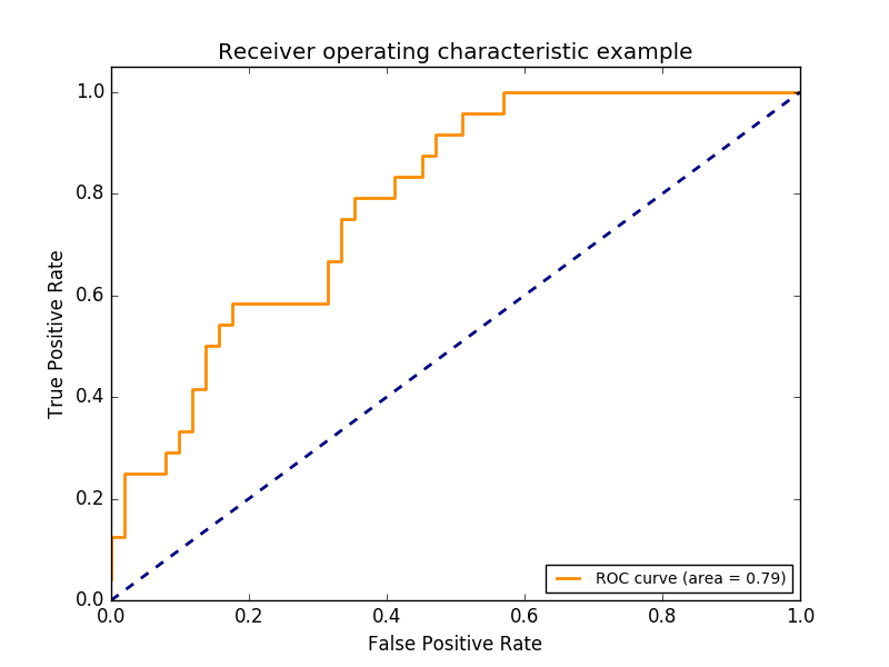
roc_auc_score The function is the receiver operating characteristic (ROC) represented by AUC or AUROC. ) Calculate the area under the curve. By calculating the area under the roc curve, the curve information is combined into one number. For more information, see Wikipedia article on AUC.
>>> import numpy as np
>>> from sklearn.metrics import roc_auc_score
>>> y_true = np.array([0, 0, 1, 1])
>>> y_scores = np.array([0.1, 0.4, 0.35, 0.8])
>>> roc_auc_score(y_true, y_scores)
0.75
In multi-label classification, the roc_auc_score function is extended by averaging the labels as described above. ROC does not require optimizing the threshold for each label compared to metrics such as subset accuracy, humming loss, and F1 score. You can also use the roc_auc_score function in a multiclass classification if the predicted output has been binary evolved.
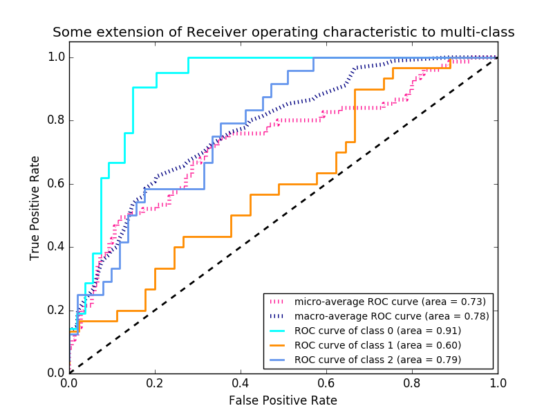
--Example: --For an example of using ROC to evaluate the output quality of a classifier, see Receiver Operating Characteristic (ROC) (http://scikit-learn.org/0.18/auto_examples/model_selection/plot_roc.html#sphx). See (-glr-auto-examples-model-selection-plot-roc-py). --For an example of using ROC to evaluate the output quality of classifiers using cross-validation, see Recipient Operating Characteristic (ROC) by Cross-Validation. auto_examples / model_selection / plot_roc_crossval.html # sphx-glr-auto-examples-model-selection-plot-roc-crossval-py). --For an example of using ROC to model a species distribution, see Species Distribution Model (http://scikit-learn.org/0.18/auto_examples/applications/plot_species_distribution_modeling.html#sphx-glr-auto- See examples-applications-plot-species-distribution-modeling-py).
3.3.2.13. 0-1 loss
zero_one_loss The function is 0- for $ n_ {\ text {samples}} $ 1 Calculate the sum or average of the classification loss $ (L_ {0-1}) $. By default, the function is normalized to the sample. To find the sum of $ L_ {0-1} $, set normalize to False.
For multi-label classification, zero_one_loss scores a subset as 1 if the label exactly matches the prediction, and as zero if there is an error. By default, this function returns the percentage of an incompletely predicted subset. To get the number of such subsets instead, set normalize to False
If $ \ hat {y} i $ is the predicted value for the $ i $ th sample and $ y_i $ is the corresponding true value, then the 0-1 loss $ L {0-1} $ is Is defined in.
L_{0-1}(y_i, \hat{y}_i) = 1(\hat{y}_i \not= y_i)
Where $ 1 (x) $ is the Indicator Function (https://en.wikipedia.org/wiki/Indicator_function).
>>> from sklearn.metrics import zero_one_loss
>>> y_pred = [1, 2, 3, 4]
>>> y_true = [2, 2, 3, 4]
>>> zero_one_loss(y_true, y_pred)
0.25
>>> zero_one_loss(y_true, y_pred, normalize=False)
1
For multi-labels with a binary label indicator, there is an error in the first label set [0,1].
>>>
>>> zero_one_loss(np.array([[0, 1], [1, 1]]), np.ones((2, 2)))
0.5

>>> zero_one_loss(np.array([[0, 1], [1, 1]]), np.ones((2, 2)),  normalize=False)
1
--Example: --For an example of zero loss for removing recursive features using cross-validation, see Recursive Feature Removal by Cross Validation (http://scikit-learn.org/0.18/auto_examples) See /feature_selection/plot_rfe_with_cross_validation.html#sphx-glr-auto-examples-feature-selection-plot-rfe-with-cross-validation-py).
3.3.2.14. Brier score loss
The brier_score_loss function is a binary class Brier score .wikipedia.org/wiki/Brier_score) is calculated. Quote Wikipedia:
The Brier score is a good score function that measures the accuracy of stochastic predictions. It can be applied to tasks where predictions need to assign probabilities to a set of mutually exclusive discrete results.
This function returns the score of the mean square difference between the actual result and the expected probability of a possible result. The actual result must be 1 or 0 (true or false), but the predicted probability of the actual result is between 0 and 1. The loss of brier score is also 0 to 1, and the lower the score (the smaller the mean squares), the more accurate the prediction. This can be thought of as a measure of the "range measurement" of a set of stochastic predictions.
BS = \frac{1}{N} \sum_{t=1}^{N}(f_t - o_t)^2
Where $ N $ is the total number of predictions and $ f_t $ is the predicted probability of the actual result $ o_t $.
Here's a small example of how to use this function ::
>>> import numpy as np
>>> from sklearn.metrics import brier_score_loss
>>> y_true = np.array([0, 1, 1, 0])
>>> y_true_categorical = np.array(["spam", "ham", "ham", "spam"])
>>> y_prob = np.array([0.1, 0.9, 0.8, 0.4])
>>> y_pred = np.array([0, 1, 1, 0])
>>> brier_score_loss(y_true, y_prob)
0.055
>>> brier_score_loss(y_true, 1-y_prob, pos_label=0)
0.055
>>> brier_score_loss(y_true_categorical, y_prob, pos_label="ham")
0.055
>>> brier_score_loss(y_true, y_prob > 0.5)
0.0
--Example: --For an example of using the Brier score loss to perform a classifier stochastic range measurement, see Classifier Probabilistic Range Measurement (http://scikit-learn.org/0.18/auto_examples/calibration/plot_calibration. See html # sphx-glr-auto-examples-calibration-plot-calibration-py). --Reference: --G. Brier, Verification of Probabilistically Expressed Forecasts, Monthly Weather Assessment 78.1 (1950)
3.3.3. Multi-label ranking metric
With multi-label learning, each sample can have any number of ground true labels associated with it. The goal is to give a high score and rank the truth price tag on the ground.
3.3.3.1. Coverage error
coverage_error The function is final so that all true labels are predicted. Calculate the average number of labels that must be included in a predictive forecast. This is useful if you want to know how many top score labels you have to predict on average without losing their true value. Therefore, the best value for this metric is the average number of true labels. Formally, given the binary indicator matrix for ground truth labels and the score associated with each label, coverage is defined as:
Officially, the ground truth label $ y \ in \ left \\ {0, 1 \ right \} ^ {n \ _ \ text {samples} \ times n \ _ \ text {labels}} $ 2 Given the base indicator matrix and the score associated with each label $ \ hat {f} \ in \ mathbb {R} ^ {n \ _ \ text {samples} \ times n \ _ \ text {labels}} $ , Coverage
coverage(y, \hat{f}) = \frac{1}{n_{\text{samples}}}
  \sum_{i=0}^{n_{\text{samples}} - 1} \max_{j:y_{ij} = 1} \text{rank}_{ij}
soy_scoresThe ties are broken by giving the maximum rank assigned to all the ties.
Here's a small example of how to use this function ::
>>> import numpy as np
>>> from sklearn.metrics import coverage_error
>>> y_true = np.array([[1, 0, 0], [0, 0, 1]])
>>> y_score = np.array([[0.75, 0.5, 1], [1, 0.2, 0.1]])
>>> coverage_error(y_true, y_score)
2.5
3.3.3.2. Average label rank conformance rate
The label_ranking_average_precision_score function implements Label Rank Average Conformance (LRAP). This metric is linked to the average_precision_score function, but with precision and recall. It is based on the concept of label ranking instead of. Label Rank Mean Accuracy (LRAP) is the average value of each Grand Truth Label assigned to each sample and is the ratio of true and total labels with a low score. This metric will improve your score if you can increase the rank of the label associated with each sample. The score obtained is always exactly greater than 0, with the best value being 1. If there is exactly one associated label per sample, the average label ranking match rate corresponds to the Average Reciprocal Rank (https://en.wikipedia.org/wiki/Mean_reciprocal_rank). Formally, the two-item index matrix of the ground truth table $ \ mathcal {R} ^ {n_ \ text {samples} \ times n_ \ text {labels}} $ and each label $ \ hat {f} \ In mathcal {R} ^ {n_ \ text {samples} \ times n_ \ text {labels}} $, the mean precision is defined as:
LRAP(y, \hat{f}) = \frac{1}{n_{\text{samples}}}
  \sum_{i=0}^{n_{\text{samples}} - 1} \frac{1}{|y_i|}
  \sum_{j:y_{ij} = 1} \frac{|\mathcal{L}_{ij}|}{\text{rank}_{ij}}
>>> import numpy as np
>>> from sklearn.metrics import label_ranking_average_precision_score
>>> y_true = np.array([[1, 0, 0], [0, 0, 1]])
>>> y_score = np.array([[0.75, 0.5, 1], [1, 0.2, 0.1]])
>>> label_ranking_average_precision_score(y_true, y_score)
0.416...
3.3.3.3. Ranking loss
The label_ranking_loss function is the number of misordered label pairs, or true labels. Calculates a ranking loss that averages the number of label pairs that have a lower score than the fake label and are weighted by the inverse of the fake label and the true label. The lowest achievable ranking loss is zero. The formula is 2 of the ground truth label $ y \ in \ left \\ {0, 1 \ right \} \ ^ {n \ _ \ text {samples} \ times n \ _ \ text {labels}} $ Given the base indicator matrix and the score associated with each label $ \ hat {f} \ in \ mathbb {R} ^ {n \ _ \ text {samples} \ times n \ _ \ text {labels}} $ If the ranking loss is
\text{ranking\_loss}(y, \hat{f}) =  \frac{1}{n_{\text{samples}}}
  \sum_{i=0}^{n_{\text{samples}} - 1} \frac{1}{|y_i|(n_\text{labels} - |y_i|)}
  \left|\left\{(k, l): \hat{f}_{ik} < \hat{f}_{il}, y_{ik} = 1, y_{il} = 0 \right\}\right|
here,$ |\cdot|
An example of using this function is shown below.
>>> import numpy as np
>>> from sklearn.metrics import label_ranking_loss
>>> y_true = np.array([[1, 0, 0], [0, 0, 1]])
>>> y_score = np.array([[0.75, 0.5, 1], [1, 0.2, 0.1]])
>>> label_ranking_loss(y_true, y_score)
0.75...
>>> # With the following prediction, we have perfect and minimal loss
>>> y_score = np.array([[1.0, 0.1, 0.2], [0.1, 0.2, 0.9]])
>>> label_ranking_loss(y_true, y_score)
0.0
3.3.4. Regression metric
sklearn.metrics Modules have some losses, scores, and utilities for measuring regression performance. Implements the function. mean_squared_error, mean_absolute_error /modules/generated/sklearn.metrics.mean_absolute_error.html#sklearn.metrics.mean_absolute_error), [explain_variance_score](http://scikit-learn.org/0.18/modules/generated/sklearn.metrics.explained_variance_score.html#sklearn. Handles multiple output cases, such as metrics.explained_variance_score) and r2_score Some have been extended to do.
These functions have a multioutput keyword argument that specifies how to average the scores or losses for individual targets. The default is 'uniform_average'. This specifies a uniformly weighted average for the output. If a ndarray with a shape of(n_outputs,)is passed, the entry is interpreted as a weight and a weighted average is returned accordingly. If multioutput is'raw_values', all individual scores and losses that have not changed are returned as an array of shapes (n_outputs,).
r2_score and explain_variance_score accept an additional value 'variance_weighted' for the multioutput parameter. This option leads to weighting of individual scores by the variance of the corresponding target variable. This setting quantifies the globally captured unscaled variance. If the target variables are on different scales, this score is important to better explain that the variance variables are high. multioutput ='variance_weighted' is the default value for r2_score for backward compatibility. This will change to 'uniform_average' in the future.
3.3.4.1. Explanatory variable score
explain_variance_score is Explanatory Variable Regression Score .org / wiki / Explained_variation) is calculated. If $ \ hat {y} $ is the estimated target output, $ y $ is the corresponding (correct) target output, and $ Var $ is the variance that is the square of the standard deviation, then the explanatory variables are: Is estimated as.
\texttt{explained_variance}(y, \hat{y}) = 1 - \frac{Var\{ y - \hat{y}\}}{Var\{y\}}
The highest score is 1.0, the lower the value, the worse. The following is an example of using the explain_variance_score function.
>>> from sklearn.metrics import explained_variance_score
>>> y_true = [3, -0.5, 2, 7]
>>> y_pred = [2.5, 0.0, 2, 8]
>>> explained_variance_score(y_true, y_pred)
0.957...
>>> y_true = [[0.5, 1], [-1, 1], [7, -6]]
>>> y_pred = [[0, 2], [-1, 2], [8, -5]]
>>> explained_variance_score(y_true, y_pred, multioutput='raw_values')
...
array([ 0.967...,  1.        ])
>>> explained_variance_score(y_true, y_pred, multioutput=[0.3, 0.7])
...
0.990...
3.3.4.2. Average absolute error
mean_absolute_error The function is mean absolute error. .org / wiki / Mean_absolute_error), calculate the risk metric corresponding to the expected value of absolute error loss or $ l1 $ norm loss. If $ \ hat {y} \ _i $ is the predicted value for the $ i $ th sample and $ y \ _i $ is the corresponding true value, then $ n \ _ {\ text {samples}} $ The estimated mean absolute error (MAE) is defined as:
\text{MAE}(y, \hat{y}) = \frac{1}{n_{\text{samples}}} \sum_{i=0}^{n_{\text{samples}}-1} \left| y_i - \hat{y}_i \right|.
The following is an example of using the mean_absolute_error function.
>>> from sklearn.metrics import mean_absolute_error
>>> y_true = [3, -0.5, 2, 7]
>>> y_pred = [2.5, 0.0, 2, 8]
>>> mean_absolute_error(y_true, y_pred)
0.5
>>> y_true = [[0.5, 1], [-1, 1], [7, -6]]
>>> y_pred = [[0, 2], [-1, 2], [8, -5]]
>>> mean_absolute_error(y_true, y_pred)
0.75
>>> mean_absolute_error(y_true, y_pred, multioutput='raw_values')
array([ 0.5,  1. ])
>>> mean_absolute_error(y_true, y_pred, multioutput=[0.3, 0.7])
...
0.849...
3.3.4.3. Mean squared error
mean_squared_error The function is a squared (secondary) error loss or expected value of loss. Calculate the corresponding risk metric, Mean Squared Error (https://en.wikipedia.org/wiki/Mean_squared_error). If $ \ hat {y} \ _i $ is the predicted value for the $ i $ th sample and $ y \ _i $ is the corresponding true value, then $ n \ _ {\ text {samples}} $ The estimated mean squared error (MSE) is defined as:
\text{MSE}(y, \hat{y}) = \frac{1}{n_\text{samples}} \sum_{i=0}^{n_\text{samples} - 1} (y_i - \hat{y}_i)^2.
The following is an example of using the mean_squared_error function.
>>> from sklearn.metrics import mean_squared_error
>>> y_true = [3, -0.5, 2, 7]
>>> y_pred = [2.5, 0.0, 2, 8]
>>> mean_squared_error(y_true, y_pred)
0.375
>>> y_true = [[0.5, 1], [-1, 1], [7, -6]]
>>> y_pred = [[0, 2], [-1, 2], [8, -5]]
>>> mean_squared_error(y_true, y_pred)
0.7083...
--Example: --For an example of using the squared mean error to evaluate gradient boosting regression, see Gradient Boost Regression (http://scikit-learn.org/0.18/auto_examples/ensemble/plot_gradient_boosting_regression.html#sphx-glr-auto). See -examples-ensemble-plot-gradient-boosting-regression-py).
3.3.4.4. Central absolute error
median_absolute_error is especially interesting because it is robust against outliers. The loss is calculated by taking the median of all absolute differences between the target and the forecast. If $ \ hat {y} \ _i $ is the predicted value for the $ i $ th sample and $ y \ _i $ is the corresponding true value, then $ n \ _ {\ text {samples}} $ The estimated median absolute error (MedAE) is defined as:
\text{MedAE}(y, \hat{y}) = \text{median}(\mid y_1 - \hat{y}_1 \mid, \ldots, \mid y_n - \hat{y}_n \mid).
median_absolute_error does not support multi-output. The following is an example of using the median_absolute_error function.
>>> from sklearn.metrics import median_absolute_error
>>> y_true = [3, -0.5, 2, 7]
>>> y_pred = [2.5, 0.0, 2, 8]
>>> median_absolute_error(y_true, y_pred)
0.5
3.3.4.5. R² score, coefficient of determination
r2_score The function is the coefficient of determination (https://en.wikipedia. org / wiki / Coefficient_of_determination) Calculates R². This provides an indicator that future samples are likely to be predicted by the model. The highest possible score is 1.0 and can be negative (because the model can deteriorate arbitrarily). In a constant model that ignores input features and always predicts the expected value of y, the R ^ 2 score is 0.0. If $ \ hat {y} \ _i $ is the predicted value for the $ i $ th sample and $ y \ _i $ is the corresponding true value, then $ n \ _ {\ text {samples}} $ The estimated score R² is defined as:
R^2(y, \hat{y}) = 1 - \frac{\sum_{i=0}^{n_{\text{samples}} - 1} (y_i - \hat{y}_i)^2}{\sum_{i=0}^{n_\text{samples} - 1} (y_i - \bar{y})^2}
$ \ bar {y} = \ frac {1} {n_ {\ text {samples}}} \ sum_ {i = 0} ^ {n_ {\ text {samples}} --1} y_i $. The following is an example of using the r2_score function.
>>> from sklearn.metrics import r2_score
>>> y_true = [3, -0.5, 2, 7]
>>> y_pred = [2.5, 0.0, 2, 8]
>>> r2_score(y_true, y_pred)
0.948...
>>> y_true = [[0.5, 1], [-1, 1], [7, -6]]
>>> y_pred = [[0, 2], [-1, 2], [8, -5]]
>>> r2_score(y_true, y_pred, multioutput='variance_weighted')
...
0.938...
>>> y_true = [[0.5, 1], [-1, 1], [7, -6]]
>>> y_pred = [[0, 2], [-1, 2], [8, -5]]
>>> r2_score(y_true, y_pred, multioutput='uniform_average')
...
0.936...
>>> r2_score(y_true, y_pred, multioutput='raw_values')
...
array([ 0.965...,  0.908...])
>>> r2_score(y_true, y_pred, multioutput=[0.3, 0.7])
...
0.925...
--Example: --For an example of using the R² score to evaluate Lasso and Elastic Net on sparse signals, see Lasso and Elastic Net for Sparse Signals (http://scikit-learn.org/0.18/auto_examples/linear_model/plot_lasso_and_elasticnet). See .html # sphx-glr-auto-examples-linear-model-plot-lasso-and-elasticnet-py).
3.3.5. Clustering metric
The sklearn.metrics module implements some loss, score, and utility functions. For more information, see the Clustering Performance Evaluation section of instance clustering (http://scikit-learn.org/0.18/modules/clustering.html#clustering-evaluation) and the Biclustering Evaluation of Biclustering (http: //: //). See scikit-learn.org/0.18/modules/biclustering.html#biclustering-evaluation).
3.3.6. Dummy estimate
When doing supervised learning, a simple health check consists of comparing the estimator with a simple rule of thumb. DummyClassifier implements some of these simple strategies for classification. doing.
--stratified generates random predictions by respecting the training set class distribution.
--most_frequent always predicts the most frequent labels in the training set.
--prior always predicts the class that maximizes class (like most_frequent), and predict_proba returns the class first.
--ʻUniform will randomly generate uniform predictions. --constant` ** always returns a user-provided constant label as a prediction. ** **
--The main motivation for this method is F1 scoring when the positive class is in the minority.
In all these strategies, the predict method completely ignores the input data.
To explain DummyClassifier, let's first create an imbalanced dataset:
>>> from sklearn.datasets import load_iris
>>> from sklearn.model_selection import train_test_split
>>> iris = load_iris()
>>> X, y = iris.data, iris.target
>>> y[y != 1] = -1
>>> X_train, X_test, y_train, y_test = train_test_split(X, y, random_state=0)
Next, let's compare the precision of SVC and most_frequent.
>>> from sklearn.dummy import DummyClassifier
>>> from sklearn.svm import SVC
>>> clf = SVC(kernel='linear', C=1).fit(X_train, y_train)
>>> clf.score(X_test, y_test)
0.63...
>>> clf = DummyClassifier(strategy='most_frequent',random_state=0)
>>> clf.fit(X_train, y_train)
DummyClassifier(constant=None, random_state=0, strategy='most_frequent')
>>> clf.score(X_test, y_test)
0.57...
We find that SVC is not much better than a dummy classifier. Now let's change the kernel:
>>> clf = SVC(kernel='rbf', C=1).fit(X_train, y_train)
>>> clf.score(X_test, y_test)
0.97...
The accuracy has improved to almost 100%. If the CPU cost is not very high, cross-validation is recommended for a more accurate assessment of accuracy. For more information, see the Cross-validation: Estimated Performance Evaluation (http://qiita.com/nazoking@github/items/13b167283590f512d99a) section. In addition, it is highly recommended to use the appropriate method when optimizing the parameter space. See the Estimator Hyperparameter Tuning (http://scikit-learn.org/0.18/modules/grid_search.html#grid-search) section for more information. More generally, if the classifier's accuracy is too close to random, something could be wrong. Features are useless, hyperparameters are not adjusted correctly, classifiers are suffering from class imbalances, etc.
DummyRegressor also implements four simple rules of thumb for regression. I am.
--mean always predicts the average training goal.
--median always predicts the median training goal.
--quantile always predicts that the user will provide the quantile of the training goal.
--constant always returns a constant value provided by the user as a prediction.
In all of these strategies, the predict method completely ignores the input data.
[scikit-learn 0.18 User Guide 3. Model Selection and Evaluation](http://qiita.com/nazoking@github/items/267f2371757516f8c168#3-%E3%83%A2%E3%83%87%E3%83] From% AB% E3% 81% AE% E9% 81% B8% E6% 8A% 9E% E3% 81% A8% E8% A9% 95% E4% BE% A1)
© 2010 --2016, scikit-learn developers (BSD license).