[PYTHON] 100 Language Processing Knock 2020 Chapter 8: Neural Net

The other day, Language Processing 100 Knock 2020 was released. I myself have only been in natural language processing for a year, and I don't know the details, but I will solve all the problems and publish them in order to improve my technical skills.

All shall be executed on jupyter notebook, and the restrictions of the problem statement may be broken conveniently. The source code is also on github. Yes.

Chapter 7 is here.

The environment is Python 3.8.2 and Ubuntu 18.04.

Chapter 8: Neural Net

Implement a categorization model with a neural network based on the categorization of news articles discussed in Chapter 6. In this chapter, use machine learning platforms such as PyTorch, TensorFlow, and Chainer.

Use PyTorch.

70. Features by sum of word vectors

I want to convert the training data, validation data, and evaluation data constructed in Problem 50 into matrices and vectors. For example, for training data, we want to create a matrix $ X $ in which the feature vectors of all cases are arranged and a matrix (vector) $ Y $ in which the correct label is arranged.

X = \begin{pmatrix} \boldsymbol{x}_1 \ \boldsymbol{x}_2 \ \dots \ \boldsymbol{x}_n \ \end{pmatrix} \in \mathbb{R}^{n \times d}, Y = \begin{pmatrix} y_1 \ y_2 \ \dots \ y_n \ \end{pmatrix} \in \mathbb{N}^{n}

>
 > Here, $ n $ is the number of cases of training data, and $ \ boldsymbol x_i \ in \ mathbb {R} ^ d $ and $ y_i \ in \ mathbb N $ are $ i \ in \ {1, respectively. \ dots, n \} Represents the feature vector and correct label of the $ th case.
 > This time, there are four categories, "business", "science and technology", "entertainment", and "health". If $ \ mathbb N_4 $ represents a natural number (including $ 0 $) less than $ 4 $, the correct label $ y_i $ in any case can be represented by $ y_i \ in \ mathbb N_4 $.
 > In the following, the number of label types is represented by $ L $ ($ L = 4 $ in this classification task).
>
 > The feature vector $ \ boldsymbol x_i $ of the $ i $ th case is calculated by the following equation.
>
> $$\boldsymbol x_i = \frac{1}{T_i} \sum_{t=1}^{T_i} \mathrm{emb}(w_{i,t})$$
>
 > Here, the $ i $ th case is $ T_i $ word strings (in the article headline) $ (w_ {i, 1}, w_ {i, 2}, \ dots, w_ {i, T_i}) $ \\ mathrm {emb} (w) \ in \ mathbb {R} ^ d $ is a word vector (the number of dimensions is $ d $) corresponding to the word $ w $. That is, $ \ boldsymbol x_i $ is the article headline of the $ i $ th case expressed by the average of the vector of words included in the headline. This time, the word vector downloaded in question 60 should be used. Since we used a word vector of $ 300 $ dimension, $ d = 300 $.
 > The label $ y_i $ of the $ i $ th case is defined as follows.
>
>```math
y_i = \begin{cases}
0 & (\mbox{article}\boldsymbol x_i\mbox{If is in the "Business" category}) \\
1 & (\mbox{article}\boldsymbol x_i\mbox{Is in the "Science and Technology" category}) \\
2 & (\mbox{article}\boldsymbol x_i\mbox{If is in the "Entertainment" category}) \\
3 & (\mbox{article}\boldsymbol x_i\mbox{If is in the "health" category}) \\
\end{cases}

If there is a one-to-one correspondence between the category name and the label number, the correspondence does not have to be as shown in the above formula.

Based on the above specifications, create the following matrix / vector and save it in a file.

• Feature matrix of training data: $ X_ {\ rm train} \ in \ mathbb {R} ^ {N_t \ times d} $
• Training data label vector: $ Y_ {\ rm train} \ in \ mathbb {N} ^ {N_t} $
• Feature matrix of validation data: $ X_ {\ rm valid} \ in \ mathbb {R} ^ {N_v \ times d} $
• Validation data label vector: $ Y_ {\ rm valid} \ in \ mathbb {N} ^ {N_v} $
• Evaluation data feature matrix: $ X_ {\ rm test} \ in \ mathbb {R} ^ {N_e \ times d} $
• Evaluation data label vector: $ Y_ {\ rm test} \ in \ mathbb {N} ^ {N_e} $

Note that $ N_t, N_v, and N_e $ are the number of cases of training data, the number of cases of verification data, and the number of cases of evaluation data, respectively.

The problem statement is long and it is difficult to correct TeX.

code

import re
import spacy

Divide into words.

code

nlp = spacy.load('en')
categories = ['b', 't', 'e', 'm']
category_names = ['business', 'science and technology', 'entertainment', 'health']

code

def tokenize(x):
    x = re.sub(r'\s+', ' ', x)
    x = nlp.make_doc(x)
    x = [d.text for d in x]
    return x

def read_feature_dataset(filename):
    with open(filename) as f:
        dataset = f.read().splitlines()
    dataset = [line.split('\t') for line in dataset]
    dataset_t = [categories.index(line[0]) for line in dataset]
    dataset_x = [tokenize(line[1]) for line in dataset]
    return dataset_x, dataset_t

code

train_x, train_t = read_feature_dataset('data/train.txt')
valid_x, valid_t = read_feature_dataset('data/valid.txt')
test_x, test_t = read_feature_dataset('data/test.txt')

Convert to a feature vector.

code

import torch
from gensim.models import KeyedVectors

code

model = KeyedVectors.load_word2vec_format('../GoogleNews-vectors-negative300.bin.gz', binary=True)

code

def sent_to_vector(sent):
    lst = [torch.tensor(model[token]) for token in sent if token in model]
    return sum(lst) / len(lst)

def dataset_to_vector(dataset):
    return torch.stack([sent_to_vector(x) for x in dataset])

code

train_v = dataset_to_vector(train_x)
valid_v = dataset_to_vector(valid_x)
test_v = dataset_to_vector(test_x)

code

train_v[0]

output

tensor([ 9.0576e-02,  5.4932e-02, -7.7393e-02,  1.1810e-01, -3.8849e-02,
        -2.6074e-01, -6.4484e-02,  3.2715e-02,  1.1792e-01, -3.4363e-02,
        -1.5137e-02, -1.7090e-02,  7.2632e-02,  1.0742e-02,  1.1194e-01,
         5.8945e-02,  1.6275e-01,  1.5393e-01,  7.0496e-02, -1.5210e-01,
         2.8320e-02,  1.1719e-02,  1.9702e-01, -1.5610e-02, -2.3438e-02,
         1.8921e-02,  2.8687e-02, -2.3438e-02,  2.3315e-02, -5.7480e-02,
         2.1973e-03, -1.0449e-01, -9.7534e-02, -1.3694e-01,  1.6144e-01,
        -2.6062e-02,  3.1250e-02,  1.9482e-01, -1.0788e-01,  7.2571e-02,
        -1.3916e-02,  1.1121e-01,  7.0801e-03, -4.1016e-02, -1.9580e-01,
         1.7334e-02,  1.0986e-02, -6.9485e-03,  9.2773e-02,  7.2205e-02,
         6.8298e-02, -5.3589e-02, -1.7447e-01,  1.0245e-01, -8.6426e-02,
        -9.0942e-03, -1.7212e-01, -1.3789e-01, -1.0355e-01,  1.9226e-02,
         1.0620e-02,  9.7626e-02, -5.1147e-02,  1.1371e-01,  3.5156e-02,
        -4.8523e-03, -7.1960e-02,  1.1841e-01, -1.0974e-01,  1.2878e-01,
        -7.3273e-02,  5.3711e-02,  9.6313e-02, -9.0950e-02,  4.3335e-02,
        -4.7424e-02, -3.0518e-02,  5.2856e-02,  3.7842e-02,  2.2559e-01,
         4.0161e-02, -2.3822e-01, -1.3531e-01, -3.8513e-02, -1.1475e-02,
        -7.3242e-02, -1.9324e-01,  1.9553e-01,  1.0870e-01,  1.5405e-01,
         2.8793e-02, -1.9226e-01,  3.1952e-02, -1.0471e-01,  4.9561e-02,
         6.5918e-03, -5.6793e-02,  1.8628e-01, -5.5908e-02, -9.8999e-02,
        -2.1448e-01, -1.6602e-02,  6.7627e-02,  2.1149e-02, -6.8970e-02,
         2.3804e-03, -2.1729e-02, -9.1599e-02, -8.7585e-02, -1.1963e-01,
        -8.7555e-02,  6.1768e-02, -1.6205e-02,  2.9572e-02,  1.2207e-04,
         1.3300e-01,  1.6541e-02, -1.3672e-01,  1.4978e-01, -4.8828e-03,
        -2.6172e-01,  3.9093e-02,  1.4761e-01,  1.3745e-01,  8.6670e-03,
        -1.0797e-01,  8.3801e-02,  3.2690e-01, -6.9336e-02,  6.8115e-02,
         1.0571e-01, -1.2269e-01, -1.4209e-01,  7.7923e-02, -1.6113e-02,
        -6.8039e-02,  1.2909e-02, -4.9911e-02,  2.0142e-01,  9.5764e-02,
         8.1078e-02, -2.6733e-02, -1.4606e-01, -1.0449e-01,  7.1014e-02,
         9.4604e-03,  9.6436e-02, -3.3386e-02, -6.5552e-02, -4.0009e-02,
         2.0976e-01, -9.5825e-02,  1.2494e-01, -1.1230e-02,  1.3062e-02,
         1.8829e-02, -1.7525e-01, -1.6845e-01, -3.0334e-02, -5.6152e-02,
        -2.3193e-02, -8.4961e-02,  4.6021e-02,  1.5533e-01, -2.4780e-02,
        -1.7255e-01, -2.9472e-02, -3.2959e-03, -3.2166e-02,  1.1292e-01,
        -5.0537e-02,  6.0730e-02,  1.8042e-01, -2.6678e-01,  6.5601e-02,
        -2.4567e-01, -4.1382e-02, -2.4902e-02, -7.3853e-02,  3.8330e-02,
        -3.5229e-01, -4.8477e-02,  7.8522e-02,  2.4719e-03, -1.1414e-02,
        -8.9661e-02, -2.4341e-01,  4.9133e-02, -2.7954e-02,  9.2651e-02,
        -4.8340e-02, -5.2063e-02,  5.5817e-02, -3.7842e-03, -1.6852e-01,
         9.8267e-03,  2.1698e-02, -6.5107e-02,  9.8053e-02, -3.6621e-03,
        -2.2009e-01,  1.1389e-01,  5.0537e-02, -1.4322e-01, -8.2336e-02,
        -5.0507e-02, -2.2461e-02, -9.4971e-02, -1.0464e-01, -2.0959e-01,
        -1.2964e-01, -1.0208e-02, -4.0894e-03, -1.4893e-02, -4.9637e-02,
         6.3507e-02, -8.5968e-02,  2.3340e-01,  1.2207e-01, -1.6663e-01,
        -1.6541e-01,  6.9924e-02,  2.4414e-02, -3.3630e-02, -2.2583e-02,
        -2.1289e-01,  8.4106e-02,  1.1916e-01, -1.9623e-02, -3.2654e-02,
        -3.2394e-02,  1.5515e-01, -7.9224e-02, -9.1919e-02, -6.3782e-03,
        -3.6926e-02,  8.0456e-02, -4.5288e-02,  1.9531e-02,  7.4951e-02,
        -8.0195e-02, -2.5232e-01,  1.0986e-01, -1.2573e-01, -1.0083e-01,
         2.0972e-01,  1.3380e-03,  2.2363e-01, -6.7322e-02, -6.3477e-02,
        -2.1167e-01,  5.0659e-03, -3.2227e-02, -2.0752e-02,  2.2107e-01,
        -2.4243e-01,  1.4246e-01,  1.4465e-01, -2.0691e-01, -1.0516e-01,
        -1.0327e-01,  1.6028e-01, -1.4748e-02, -1.9310e-02,  2.3193e-02,
         1.5234e-01,  2.2034e-02, -8.0872e-04, -8.7729e-02,  5.9967e-02,
        -2.6306e-02,  1.3672e-01,  1.5301e-02,  6.3965e-02,  1.9131e-02,
        -5.8695e-02,  1.4355e-01, -9.6710e-02,  7.2235e-02, -1.0620e-02,
         6.1523e-02, -1.2626e-01,  3.3813e-02, -2.1973e-03, -1.3843e-01,
        -1.3458e-01,  5.4447e-02, -2.0325e-01,  1.2244e-01,  4.3335e-02,
        -3.1372e-02, -1.9659e-01, -1.7270e-01,  2.9846e-02, -5.8533e-02,
         6.7017e-02,  1.6748e-01,  1.1859e-01,  1.2134e-01, -1.7578e-02])

Save as pickle.

code

import pickle

code

train_t = torch.tensor(train_t).long()
valid_t = torch.tensor(valid_t).long()
test_t = torch.tensor(test_t).long()

code

with open('data/train.feature.pickle', 'wb') as f:
    pickle.dump(train_v, f)
with open('data/train.label.pickle', 'wb') as f:
    pickle.dump(train_t, f)
    
with open('data/valid.feature.pickle', 'wb') as f:
    pickle.dump(valid_v, f)
with open('data/valid.label.pickle', 'wb') as f:
    pickle.dump(valid_t, f)
    
with open('data/test.feature.pickle', 'wb') as f:
    pickle.dump(test_v, f)
with open('data/test.label.pickle', 'wb') as f:
    pickle.dump(test_t, f)

71. Prediction by single-layer neural network

Read the matrix saved in question 70 and perform the following calculations on the training data.

However, $ {\ rm softmax} $ is the softmax function, $ X_ {[1: 4]} \ in \ mathbb {R} ^ {4 \ times d} $ is the feature vector $ \ boldsymbol x_1, \ boldsymbol x_2 , \ Boldsymbol x_3, \ boldsymbol x_4 $ are arranged vertically.

The matrix $ W \ in \ mathbb {R} ^ {d \ times L} $ is a weight matrix of a single-layer neural network, which can be initialized with a random value (learned in problem 73 and later). .. Note that $ \ hat {\ boldsymbol y_1} \ in \ mathbb {N} ^ L $ is a vector representing the probability of belonging to each category when the case $ x_1 $ is classified by the unlearned matrix $ W $. Similarly, $ \ hat {Y} \ in \ mathbb {N} ^ {n \ times L} $ expresses the probabilities belonging to each category as a matrix for the training data examples $ x_1, x_2, x_3, x_4 $. are doing.

I think the questioner's intention is probably to do something like torch.empty (). Normal_ () and then F.linear (), but if you know it, it's already nn. I feel that it is okay to inherit Module. I feel the intention of the question to somehow make people who do not know what automatic differentiation is, along with the following problems.

code

import torch.nn as nn

code

class Perceptron(nn.Module):
    def __init__(self, v_size, c_size):
        super().__init__()
        self.fc = nn.Linear(v_size, c_size, bias = False)
        nn.init.xavier_normal_(self.fc.weight)
        
    def forward(self, x):
        x = self.fc(x)
        return x

code

model = Perceptron(300, 4)

code

x = model(train_v[0])
x = torch.softmax(x, dim=-1)
x

output

tensor([0.2450, 0.2351, 0.2716, 0.2483], grad_fn=<SoftmaxBackward>)

code

x = model(train_v[:4])
x = torch.softmax(x, dim=-1)
x

output

tensor([[0.2450, 0.2351, 0.2716, 0.2483],
        [0.2323, 0.2387, 0.2765, 0.2525],
        [0.2093, 0.2120, 0.2750, 0.3037],
        [0.2200, 0.2427, 0.2623, 0.2751]], grad_fn=<SoftmaxBackward>)

It has a proper probability distribution.

72. Loss and gradient calculations

Calculate the cross-entropy loss and the gradient for the matrix $ W $ for the case $ x_1 $ and the case set $ x_1, x_2, x_3, x_4 $ of the training data. For a certain case $ x_i $, the loss is calculated by the following equation.

However, the cross-entropy loss for the case set is the average of the losses of each case included in the set.

code

criterion = nn.CrossEntropyLoss()

code

y = model(train_v[:1])
t = train_t[:1]
loss = criterion(y, t)
model.zero_grad()
loss.backward()
print('loss:', loss.item())
print('Slope')
print(model.fc.weight.grad)

output

loss: 1.2622126340866089
Slope
tensor([[ 0.0229,  0.0139, -0.0196,  ...,  0.0300,  0.0307, -0.0044],
        [ 0.0219,  0.0133, -0.0187,  ...,  0.0287,  0.0294, -0.0043],
        [ 0.0201,  0.0122, -0.0172,  ...,  0.0263,  0.0270, -0.0039],
        [-0.0649, -0.0394,  0.0555,  ..., -0.0850, -0.0870,  0.0126]])

If you forget zero_grad (), the gradients will be accumulated endlessly and it will be strange.

code

model.zero_grad()
model.fc.weight.grad

output

tensor([[0., 0., 0.,  ..., 0., 0., 0.],
        [0., 0., 0.,  ..., 0., 0., 0.],
        [0., 0., 0.,  ..., 0., 0., 0.],
        [0., 0., 0.,  ..., 0., 0., 0.]])

code

y = model(train_v[:4])
t = train_t[:4]
loss = criterion(y, t)
model.zero_grad()
loss.backward()
print('loss:', loss.item())
print('Slope')
print(model.fc.weight.grad)

output

loss: 1.3049677610397339
Slope
tensor([[ 0.0044,  0.0014, -0.0114,  ...,  0.0090,  0.0150, -0.0018],
        [-0.0008,  0.0036, -0.0066,  ...,  0.0076,  0.0111, -0.0007],
        [ 0.0038,  0.0008, -0.0114,  ...,  0.0082,  0.0145, -0.0017],
        [-0.0074, -0.0059,  0.0295,  ..., -0.0248, -0.0406,  0.0042]])

73. Learning by stochastic gradient descent

Learn the matrix $ W $ using Stochastic Gradient Descent (SGD). Learning may be completed according to an appropriate standard (for example, "end at 100 epochs").

At the time of logistic regression, we used the quasi-Newton method for all the data, but this time it is a stochastic gradient descent, so we will shuffle the data set and extract it little by little.

The Dataset class is a child that has data. When __getitem__ receives an integer of the data index, the data at that address is returned.

code

class Dataset(torch.utils.data.Dataset):
    def __init__(self, x, t):
        self.x = x
        self.t = t
        self.size = len(x)
    
    def __len__(self):
        return self.size
            
    def __getitem__(self, index):
        return {
            'x':self.x[index],
            't':self.t[index],
        }

The Sampler class is a child that takes out multiple indexes of a dataset into a batch and divides the entire dataset into batches.

code

class Sampler(torch.utils.data.Sampler):
    def __init__(self, dataset, width, shuffle=False):
        self.dataset = dataset
        self.width = width
        self.shuffle = shuffle
        if not shuffle:
            self.indices = torch.arange(len(dataset))
    
    def __iter__(self):
        if self.shuffle:
            self.indices = torch.randperm(len(self.dataset))
        index = 0
        while index < len(self.dataset):
            yield self.indices[index : index + self.width]
            index += self.width

You can shuffle and retrieve the dataset by passing the Dataset and Sampler to torch.utils.data.DataLoader.

code

def gen_loader(dataset, width, sampler=Sampler, shuffle=False, num_workers=8):
    return torch.utils.data.DataLoader(
        dataset, 
        batch_sampler = sampler(dataset, width, shuffle),
        num_workers = num_workers,
    )

Prepare DataLoader with training data and verification data.

code

train_dataset = Dataset(train_v, train_t)
valid_dataset = Dataset(valid_v, valid_t)
test_dataset = Dataset(test_v, test_t)
loaders = (
    gen_loader(train_dataset, 1, shuffle = True),
    gen_loader(valid_dataset, 1),
)

Prepare a Task to calculate the loss and a Trainer to turn the optimization.

code

import torch.optim as optim

code

class Task:
    def __init__(self):
        self.criterion = nn.CrossEntropyLoss()
    
    def train_step(self, model, batch):
        model.zero_grad()
        loss = self.criterion(model(batch['x']), batch['t'])
        loss.backward()
        return loss.item()
    
    def valid_step(self, model, batch):
        with torch.no_grad():
            loss = self.criterion(model(batch['x']), batch['t'])
        return loss.item()

code

class Trainer:
    def __init__(self, model, loaders, task, optimizer, max_iter, device = None):
        self.model = model
        self.model.to(device)
        self.train_loader, self.valid_loader = loaders
        self.task = task
        self.max_iter = max_iter
        self.optimizer = optimizer
        self.device = device
    
    def send(self, batch):
        for key in batch:
            batch[key] = batch[key].to(self.device)
        return batch
        
    def train_epoch(self):
        self.model.train()
        acc = 0
        for n, batch in enumerate(self.train_loader):
            batch = self.send(batch)
            acc += self.task.train_step(self.model, batch)
            self.optimizer.step()
        return acc / n
            
    def valid_epoch(self):
        self.model.eval()
        acc = 0
        for n, batch in enumerate(self.valid_loader):
            batch = self.send(batch)
            acc += self.task.valid_step(self.model, batch)
        return acc / n
    
    def train(self):
        for epoch in range(self.max_iter):
            train_loss = self.train_epoch()
            valid_loss = self.valid_epoch()
            print('epoch {}, train_loss:{:.5f}, valid_loss:{:.5f}'.format(epoch, train_loss, valid_loss))

Perform learning.

code

model = Perceptron(300, 4)
task = Task()
optimizer = optim.SGD(model.parameters(), 0.1)
trainer = Trainer(model, loaders, task, optimizer, 10)
trainer.train()

output

epoch 0, train_loss:0.40178, valid_loss:0.32123
epoch 1, train_loss:0.29685, valid_loss:0.30087
epoch 2, train_loss:0.27381, valid_loss:0.31221
epoch 3, train_loss:0.26309, valid_loss:0.29472
epoch 4, train_loss:0.25435, valid_loss:0.29926
epoch 5, train_loss:0.24851, valid_loss:0.30723
epoch 6, train_loss:0.24424, valid_loss:0.30154
epoch 7, train_loss:0.23987, valid_loss:0.30601
epoch 8, train_loss:0.23762, valid_loss:0.30835
epoch 9, train_loss:0.23378, valid_loss:0.31116

You can see that the loss of training data has decreased.

74. Measurement of correct answer rate

When classifying the cases of training data and evaluation data using the matrix obtained in question 73, find the correct answer rate for each.

code

import numpy as np

code

class Predictor:
    def __init__(self, model, loader):
        self.model = model
        self.loader = loader
        
    def infer(self, batch):
        self.model.eval()
        return self.model(batch['x']).argmax(dim=-1).item()
        
    def predict(self):
        lst = []
        for batch in self.loader:
            lst.append(self.infer(batch))
        return lst

code

def accuracy(true, pred):
    return np.mean([t == p for t, p in zip(true, pred)])

code

predictor = Predictor(model, Loader(train_dataset, 1))
pred = predictor.predict()
print('Correct answer rate in training data:', accuracy(train_t, pred))

output

Correct answer rate in training data: 0.9239049045301385

code

predictor = Predictor(model, gen_loader(train_dataset, 1))
pred = predictor.predict()
print('Correct answer rate in training data:', accuracy(train_t, pred))

output

Correct answer rate in evaluation data: 0.8952095808383234

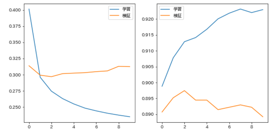
75. Loss and accuracy rate plot

By modifying the code in Q73, each time the parameter update of each epoch is completed, the loss in training data, the correct answer rate, the loss in the development data, and the correct answer rate can be plotted on a graph to check the progress of learning. Do it.

code

import matplotlib.pyplot as plt
import japanize_matplotlib
from IPython.display import clear_output

It is a code that updates the figure in real time on jupyter notebook.

code

class RealTimePlot:
    def __init__(self, legends):
        self.legends = legends
        self.fig, self.axs = plt.subplots(1, len(legends), figsize = (10, 5))
        self.lst = [[[] for _ in xs] for xs in legends]
        
    def __enter__(self):
        return self
        
    def update(self, *args):
        for i, ys in enumerate(args):
            for j, y in enumerate(ys):
                self.lst[i][j].append(y)
        clear_output(wait = True)
        for i, ax in enumerate(self.axs):
            ax.cla()
            for ys in self.lst[i]:
                ax.plot(ys)
            ax.legend(self.legends[i])
        display(self.fig)
        
    def __exit__(self, *exc_info):
        plt.close(self.fig)

code

class VerboseTrainer(Trainer):
    def accuracy(self, true, pred):
        return np.mean([t == p for t, p in zip(true, pred)])
    
    def train(self, train_v, train_t, valid_v, valid_t):
        train_loader = gen_loader(Dataset(train_v, train_t), 1)
        valid_loader = gen_loader(Dataset(valid_v, valid_t), 1)
        with RealTimePlot([['Learning', 'Verification']] * 2) as rtp:
            for epoch in range(self.max_iter):
                self.model.to(self.device)
                train_loss = self.train_epoch()
                valid_loss = self.valid_epoch()
                train_acc = self.accuracy(train_t, Predictor(self.model.cpu(), train_loader).predict())
                valid_acc = self.accuracy(valid_t, Predictor(self.model.cpu(), valid_loader).predict())
                rtp.update([train_loss, valid_loss], [train_acc, valid_acc])

Calculate the correct answer rate in Trainer, and repeat erasing and displaying on jupyter notebook.

code

model = Perceptron(300, 4)
task = Task()
optimizer = optim.SGD(model.parameters(), 0.1)
trainer = VerboseTrainer(model, loaders, task, optimizer, 10)
train_predictor = Predictor(model, gen_loader(test_dataset, 1))
valid_predictor = Predictor(model, gen_loader(test_dataset, 1))
trainer.train(train_v, train_t, valid_v, valid_t)

76. Checkpoint

Modify the code in question 75 and write the checkpoints (values of parameters in the process of learning (weight matrix, etc.) and internal state of the optimization algorithm) to a file each time the parameter update of each epoch is completed.

code

import os

code

class LoggingTrainer(Trainer):
    def save(self, epoch):
        torch.save({'epoch' : epoch, 'optimizer': self.optimizer}, f'trainer_states{epoch}.pt')
        torch.save(self.model.state_dict(), f'checkpoint{epoch}.pt')
    
    def train(self):
        for epoch in range(self.max_iter):
            train_loss = self.train_epoch()
            valid_loss = self.valid_epoch()
            self.save(epoch)
            print('epoch {}, train_loss:{:.5f}, valid_loss:{:.5f}'.format(epoch, train_loss, valid_loss))

To save the model, the dictionary of values called by state_dict () is also torch.save.

code

model = Perceptron(300, 4)
task = Task()
optimizer = optim.SGD(model.parameters(), 0.1)
trainer = LoggingTrainer(model, loaders, task, optimizer, 10)
trainer.train()

output

epoch 0, train_loss:0.40303, valid_loss:0.31214
epoch 1, train_loss:0.29639, valid_loss:0.29592
epoch 2, train_loss:0.27451, valid_loss:0.29903
epoch 3, train_loss:0.26194, valid_loss:0.29984
epoch 4, train_loss:0.25443, valid_loss:0.29787
epoch 5, train_loss:0.24855, valid_loss:0.30021
epoch 6, train_loss:0.24384, valid_loss:0.30676
epoch 7, train_loss:0.24003, valid_loss:0.30658
epoch 8, train_loss:0.23756, valid_loss:0.30995
epoch 9, train_loss:0.23390, valid_loss:0.30879

code

ls result/checkpoint*

output

result/checkpoint0.pt  result/checkpoint4.pt  result/checkpoint8.pt
result/checkpoint1.pt  result/checkpoint5.pt  result/checkpoint9.pt
result/checkpoint2.pt  result/checkpoint6.pt
result/checkpoint3.pt  result/checkpoint7.pt

code

ls result/trainer_states*

output

result/trainer_states0.pt  result/trainer_states4.pt  result/trainer_states8.pt
result/trainer_states1.pt  result/trainer_states5.pt  result/trainer_states9.pt
result/trainer_states2.pt  result/trainer_states6.pt
result/trainer_states3.pt  result/trainer_states7.pt

77. Mini batch

Modify the code in question 76, calculate the loss / gradient for each $ B $ case, and update the value of the matrix $ W $ (mini-batch). Compare the time required to learn one epoch while changing the value of $ B $ to $ 1, 2, 4, 8, \ dots $.

Mini-batch is already implemented in Dataset, so just change the width of Sampler.

code

from time import time
from contextlib import contextmanager

code

@contextmanager
def timer(description):
    start = time()
    yield
    print(description, ': {:.3f}Seconds'.format(time()-start))

code

B = [1, 2, 4, 8, 16, 32, 64, 128, 256, 512, 1024]

code

task = Task()
for b in B:
    model = Perceptron(300, 4)
    loaders = (
        gen_loader(train_dataset, b, shuffle = True),
        gen_loader(valid_dataset, 1)
    )
    optimizer = optim.SGD(model.parameters(), 0.1 * b)
    trainer = Trainer(model, loaders, task, optimizer, 3)
    with timer(f'Batch size{b}'):
        trainer.train()

output

epoch 0, train_loss:0.40374, valid_loss:0.31423
epoch 1, train_loss:0.29578, valid_loss:0.29623
epoch 2, train_loss:0.27499, valid_loss:0.29798
Batch size 1: 9.657 seconds
epoch 0, train_loss:0.39955, valid_loss:0.31440
epoch 1, train_loss:0.29591, valid_loss:0.29844
epoch 2, train_loss:0.27373, valid_loss:0.29537
Batch size 2: 5.325 seconds
epoch 0, train_loss:0.40296, valid_loss:0.31603
epoch 1, train_loss:0.29613, valid_loss:0.31031
epoch 2, train_loss:0.27469, valid_loss:0.29736
Batch size 4: 3.083 seconds
epoch 0, train_loss:0.40289, valid_loss:0.31443
epoch 1, train_loss:0.29676, valid_loss:0.30920
epoch 2, train_loss:0.27498, valid_loss:0.30645
Batch size 8: 1.982 seconds
epoch 0, train_loss:0.40211, valid_loss:0.31350
epoch 1, train_loss:0.29613, valid_loss:0.30777
epoch 2, train_loss:0.27449, valid_loss:0.29903
Batch size 16: 1.420 seconds
epoch 0, train_loss:0.40343, valid_loss:0.32170
epoch 1, train_loss:0.29695, valid_loss:0.30777
epoch 2, train_loss:0.27486, valid_loss:0.29472
Batch size 32: 1.202 seconds
epoch 0, train_loss:0.40753, valid_loss:0.32378
epoch 1, train_loss:0.29829, valid_loss:0.29770
epoch 2, train_loss:0.27663, valid_loss:0.30175
Batch size 64: 1.060 seconds
epoch 0, train_loss:0.41799, valid_loss:0.33559
epoch 1, train_loss:0.30109, valid_loss:0.30401
epoch 2, train_loss:0.27763, valid_loss:0.30351
Batch size 128: 0.906 seconds
epoch 0, train_loss:0.56407, valid_loss:0.30955
epoch 1, train_loss:0.31099, valid_loss:0.32111
epoch 2, train_loss:0.28797, valid_loss:0.29928
Batch size 256: 2.234 seconds
epoch 0, train_loss:1.19123, valid_loss:0.32315
epoch 1, train_loss:0.52350, valid_loss:0.39943
epoch 2, train_loss:0.42246, valid_loss:0.36194
Batch size 512: 1.323 seconds
epoch 0, train_loss:3.77615, valid_loss:0.60957
epoch 1, train_loss:1.05934, valid_loss:0.89198
epoch 2, train_loss:0.80346, valid_loss:0.61814
Batch size 1024: 1.057 seconds

78. Learning on GPU

Modify the code in question 77 and run the learning on the GPU.

If you put it on torch.device ('cuda'), you can get on.

code

device = torch.device('cuda')
model = Perceptron(300, 4)
task = Task()
loaders = (
    gen_loader(train_dataset, 128, shuffle = True),
    gen_loader(valid_dataset, 1),
)
optimizer = optim.SGD(model.parameters(), 0.1 * 128)
trainer = Trainer(model, loaders, task, optimizer, 3, device=device)
with timer('time'):
    trainer.train()

output

epoch 0, train_loss:0.41928, valid_loss:0.31376
epoch 1, train_loss:0.30053, valid_loss:0.29341
epoch 2, train_loss:0.27865, valid_loss:0.29917
time: 1.433 seconds

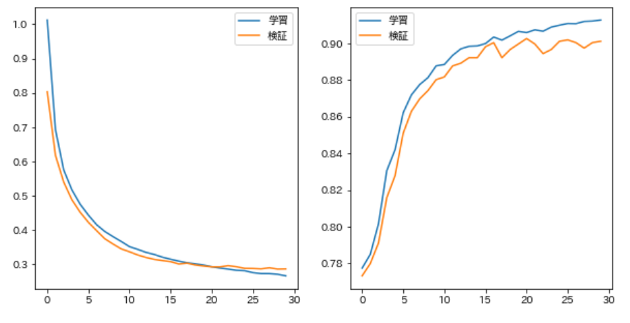
79. Multi-layer neural network

Modify the code in Problem 78 to build a high-performance categorizer while changing the shape of the neural network, such as introducing bias terms and multi-layering.

I tried to make it multi-layered, but it seems that the performance does not improve significantly by itself.

code

class ModelNLP79(nn.Module):
    def __init__(self, v_size, h_size, c_size):
        super().__init__()
        self.fc1 = nn.Linear(v_size, h_size)
        self.act = nn.ReLU()
        self.fc2 = nn.Linear(h_size, c_size)
        self.dropout = nn.Dropout(0.2)
        nn.init.kaiming_normal_(self.fc1.weight)
        nn.init.kaiming_normal_(self.fc2.weight)
        
    def forward(self, x):
        x = self.fc1(x)
        x = self.act(x)
        x = self.dropout(x)
        x = self.fc2(x)
        return x

code

model = ModelNLP79(300, 128, 4)
task = Task()
loaders = (
    gen_loader(train_dataset, 128, shuffle = True),
    gen_loader(valid_dataset, 1)
)
optimizer = optim.SGD(model.parameters(), 0.1)
trainer = VerboseTrainer(model, loaders, task, optimizer, 30, device)
trainer.train(train_v, train_t, valid_v, valid_t)

Next is Chapter 9

Language processing 100 knocks 2020 Chapter 9: RNN, CNN