[PYTHON] 100 Language Processing Knock 2020 Chapter 6: Machine Learning

The other day, 100 Language Processing Knock 2020 was released. I myself have only been in natural language processing for a year, and I don't know the details, but I will solve all the problems and publish them in order to improve my technical skills.

All shall be executed on jupyter notebook, and the restrictions of the problem statement may be broken conveniently. The source code is also on github. Yes.

Chapter 5 is here.

The environment is Python 3.8.2 and Ubuntu 18.04.

Chapter 6: Machine Learning

In this chapter, we will use the News Aggregator Data Set published by Fabio Gasparetti to work on the task (category classification) of classifying news article headlines into the categories of "business", "science and technology", "entertainment", and "health".

Please download the required dataset from here.

The downloaded file shall be placed under data.

50. Obtaining and shaping data

Download the News Aggregator Data Set and create training data (train.txt), verification data (valid.txt), and evaluation data (test.txt) as follows.

1. Unzip the downloaded zip file and read the explanation of readme.txt.
2. Extract only cases (articles) whose information sources (publishers) are "Reuters", "Huffington Post", "Businessweek", "Contactmusic.com", and "Daily Mail".
3. Randomly sort the extracted cases.
4. Divide 80% of the extracted cases into training data and the remaining 10% into verification data and evaluation data, and save them with the file names train.txt, valid.txt, and test.txt, respectively. Write one case per line in the file, and use the tab-delimited format of the category name and article headline. After creating the training data and evaluation data, check the number of cases in each category.

Read the dataset from the zip file.

code

import zipfile

code

#Read from zip file
with zipfile.ZipFile('data/NewsAggregatorDataset.zip') as f:
    with f.open('newsCorpora.csv') as g:
        data = g.read()

#Decode byte sequence
data = data.decode('UTF-8').splitlines()

#Tab delimited
data = [line.split('\t') for line in data]
len(data)

output

422937

Specify the information source and sort at random.

code

publishers = {
    'Reuters',
    'Huffington Post',
    'Businessweek',
    'Contactmusic.com',
    'Daily Mail',
}
data = [
    lst
    for lst in data
    if lst[3] in publishers
]
data.sort()
len(data)

output

13356

Discard all but the category name and article headline.

code

data = [
    [lst[4], lst[1]]
    for lst in data
]

Divide into learning / verification / evaluation data. sklearn has a function with a similar function, but it's not as difficult as trying to get into the black box. Just specify the location to cut out and cut.

code

train_end = int(len(data) * 0.8)
valid_end = int(len(data) * 0.9)
train = data[:train_end]
valid = data[train_end:valid_end]
test = data[valid_end:]
print('Training data', len(train))
print('Validation data', len(valid))
print('Evaluation data', len(test))

output

Training data 10684
Validation data 1336
Evaluation data 1336

Save to a file.

code

def write_dataset(filename, data):
    with open(filename, 'w') as f:
        for lst in data:
            print('\t'.join(lst), file = f)

code

write_dataset('../train.txt', train)
write_dataset('../valid.txt', valid)
write_dataset('../test.txt', test)

Check the number of cases for each category.

code

from collections import Counter
from tabulate import tabulate

code

categories = ['b', 't', 'e', 'm']
category_names = ['business', 'science and technology', 'entertainment', 'health']
table = [
    [name] + [freqs[cat] for cat in categories]
    for name, freqs in [
        ('train', Counter([cat for cat, _ in train])),
        ('valid', Counter([cat for cat, _ in valid])),
        ('test', Counter([cat for cat, _ in test])),
    ]
]
tabulate(table, headers = categories)

output

          b     t     e    m
-----  ----  ----  ----  ---
train  4463  1223  4277  721
valid   617   168   459   92
test    547   134   558   97

51. Feature extraction

Extract the features from the training data, verification data, and evaluation data, and save them under the file names train.feature.txt, valid.feature.txt, and test.feature.txt (this file will be reused later in question 70). To do). Write one case per line in the file, and use a space-separated format for category names and article headlines. Feel free to design the features that are likely to be useful for categorization. The minimum baseline would be an article headline converted to a word string.

It seems that tf-idf or word vector can be used, but since the darkness of feature extraction is infinitely deep, I would like to run aground in shallow water. In other words, Bag-of-Words.

code

import re
import spacy
import nltk

Divide it into word strings and make them lowercase and stem.

code

nlp = spacy.load('en')
stemmer = nltk.stem.snowball.SnowballStemmer(language='english')

def tokenize(x):
    x = re.sub(r'\s+', ' ', x)
    x = nlp.make_doc(x) # nlp(x)Because it runs other than slow tokenizer
    x = [stemmer.stem(doc.lemma_.lower()) for doc in x]
    return x

code

tokenized_train = [[cat, tokenize(line)] for cat, line in train]
tokenized_valid = [[cat, tokenize(line)] for cat, line in valid]
tokenized_test = [[cat, tokenize(line)] for cat, line in test]

Extract the token to be used as a feature.

code

#Count the frequency of appearance
counter = Counter([
    token
    for _, tokens in tokenized_train
    for token in tokens
])

#Remove high and low frequency words
vocab = [
    token
    for token, freq in counter.most_common()
    if 2 < freq < 300
]

len(vocab)

output

4790

Bi-gram is also a feature. The US and us have become the same due to lowercase letters, but if you include bi-gram, "us stock" will be effective as a feature.

code

bi_grams = Counter([
        bi_gram
        for _, sent in tokenized_train
        for bi_gram in zip(sent, sent[1:])
    ]).most_common()
bi_grams = [tup for tup, freq in bi_grams if freq > 4]
len(bi_grams)

output

3094

you save.

code

with open('result/vocab_for_news.txt', 'w') as f:
    for token in vocab:
        print(token, file = f)

code

with open('result/bi_grams_for_news.txt', 'w') as f:
    for tup in bi_grams:
        print(' '.join(tup), file = f)

All features

code

features = vocab + [' '.join(x) for x in bi_grams]
len(features)

output

7884

Extract the features and save them.

code

import numpy as np

code

vocab_dict = {x:n for n, x in enumerate(vocab)}
bi_gram_dict = {x:n for n, x in enumerate(bi_grams)}

def count_uni_gram(sent):
    lst = [0 for token in vocab]
    for token in sent:
        if token in vocab_dict:
            lst[vocab_dict[token]] += 1
    return lst

def count_bi_gram(sent):
    lst = [0 for token in bi_grams]
    for tup in zip(sent, sent[1:]):
        if tup in bi_gram_dict:
            lst[bi_gram_dict[tup]] += 1
    return lst

code

def prepare_feature_dataset(data):
    ts = [categories.index(cat) for cat, _ in data]
    xs = [
        count_uni_gram(sent) + count_bi_gram(sent)
        for _, sent in data
    ]
    return np.array(xs, dtype=np.float32), np.array(ts, dtype=np.int8)

def write_feature_dataset(filename, xs, ts):
    with open(filename, 'w') as f:
        for t, x in zip(ts, xs):
            line = categories[t] + ' ' + ' '.join([str(int(n)) for n in x])
            print(line, file = f)    

code

train_x, train_t = prepare_feature_dataset(tokenized_train)
valid_x, valid_t = prepare_feature_dataset(tokenized_valid)
test_x, test_t = prepare_feature_dataset(tokenized_test)

code

write_feature_dataset('result/train.feature.txt', train_x, train_t)
write_feature_dataset('result/valid.feature.txt', valid_x, valid_t)
write_feature_dataset('result/test.feature.txt', test_x, test_t)

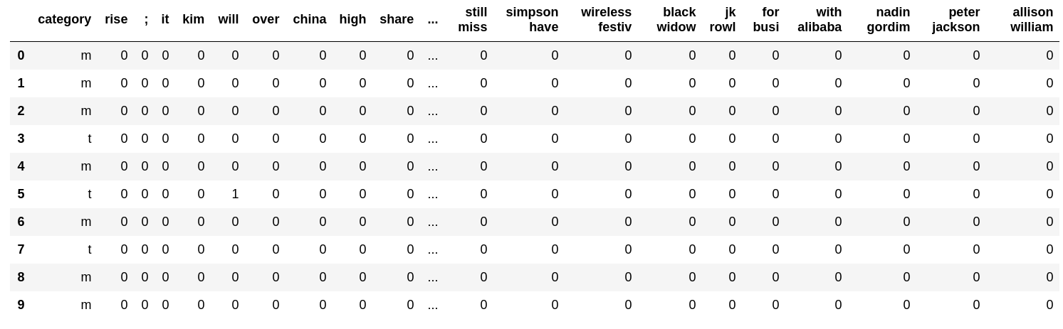
Let's look at an example.

code

import pandas as pd

code

with open('result/train.feature.txt') as f:
    table = [line.strip().split(' ') for _, line in zip(range(10), f)]
pd.DataFrame(table, columns=['category'] + features)

52. Learning

Learn the logistic regression model using the training data constructed in> 51.

Use sklearn.

It's as easy as implementing logistic regression with the steepest descent method, but if you try to scratch the quasi-Newton method, your heart will be broken by the Hessian matrix and your heart will break around the linear search, so you will have a heavy mental load on a daily basis. It is not recommended for human beings. This is an experience story, but there is a risk of running an eccentricity such as rolling the aluminum foil and stopping it where the aluminum foil conditions are met. On the other hand, scikit-learn can be used even when sleeping.

code

from sklearn.linear_model import LogisticRegression

code

lr = LogisticRegression(max_iter=1000)
lr.fit(train_x, train_t)

output

LogisticRegression(C=1.0, class_weight=None, dual=False, fit_intercept=True,
                   intercept_scaling=1, l1_ratio=None, max_iter=1000,
                   multi_class='auto', n_jobs=None, penalty='l2',
                   random_state=None, solver='lbfgs', tol=0.0001, verbose=0,
                   warm_start=False)

You can do it even if you sleep because you can make a model and fit () it. It's very easy.

53. Forecast

Use the logistic regression model learned in> 52 and implement a program that calculates the category and its prediction probability from the given article headline.

code

def predict(x):
    out = lr.predict_proba(x)
    preds = out.argmax(axis=1)
    probs = out.max(axis=1)
    return preds, probs

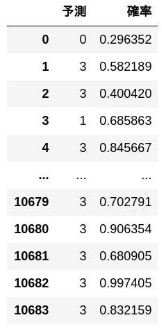
Predicted by training data.

code

preds, probs = predict(train_x)
pd.DataFrame([[y, p] for y, p in zip(preds, probs)], columns = ['Forecast', 'probability'])

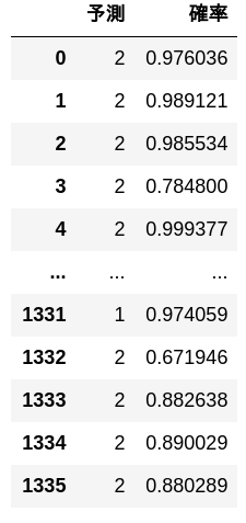
Predicted by evaluation data.

code

preds, probs = predict(test_x)
pd.DataFrame([[y, p] for y, p in zip(preds, probs)], columns = ['Forecast', 'probability'])

54. Measurement of correct answer rate

Measure the correct answer rate of the logistic regression model learned in> 52 on the training data and evaluation data.

code

def accuracy(lr, xs, ts):
    ys = lr.predict(xs)
    return (ys == ts).mean()

code

print('Training data')
print(accuracy(lr, train_x, train_t))

output

Training data
0.994664919505803

code

print('Evaluation data')
print(accuracy(lr, test_x, test_t))

output

Evaluation data
0.906437125748503

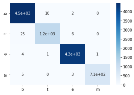
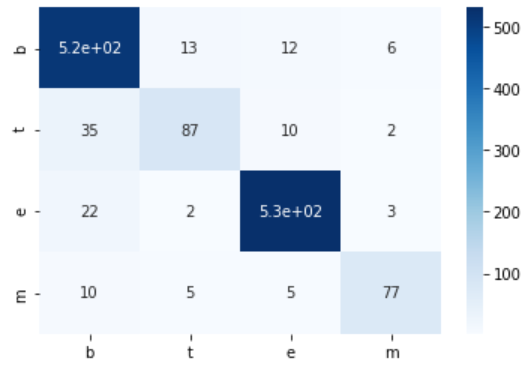
55. Creating a confusion matrix

Create a confusion matrix of the logistic regression model learned in> 52 on the training data and evaluation data.

You will be happy if you use seaborn. I think c in the confusion matrix is the sea of sea born.

code

import seaborn as sns

code

def confusion_matrix(xs, ts):
    num_class = np.unique(ts).size
    mat = np.zeros((num_class, num_class), dtype=np.int32)
    ys = lr.predict(xs)
    for y, t in zip(ys, ts):
        mat[t, y] += 1
    return mat

def show_cm(cm):
    sns.heatmap(cm, annot=True, cmap = 'Blues', xticklabels = categories, yticklabels = categories)

code

train_cm = confusion_matrix(train_x, train_t)
print('Training data')
print(train_cm)
show_cm(train_cm)

output

Training data
[[4451   10    2    0]
 [  25 1192    6    0]
 [   4    1 4271    1]
 [   5    0    3  713]]

code

test_cm = confusion_matrix(test_x, test_t)
print('Evaluation data')
print(test_cm)
show_cm(test_cm)

output

Evaluation data
[[516  13  12   6]
 [ 35  87  10   2]
 [ 22   2 531   3]
 [ 10   5   5  77]]

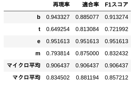
56. Measurement of precision, recall, F1 score

Measure the precision, recall, and F1 score of the logistic regression model learned in> 52 on the evaluation data. Obtain the precision rate, recall rate, and F1 score for each category, and integrate the performance for each category with the micro-average and macro-average.

There is a function that does the same processing in sklearn, but I am in a position to implement this by myself. Some tasks use the $ F_ {0.5} $ value, and I think it's better to write it yourself.

code

tp = test_cm.diagonal()
tn = test_cm.sum(axis=1) - tp
fp = test_cm.sum(axis=0) - tp

code

p = tp / (tp + tn)
r = tp / (tp + fp)
F = 2 * p * r / (p + r)

code

micro_p = tp.sum() / (tp + tn).sum()
micro_r = tp.sum() / (tp + fp).sum()
micro_F = 2 * micro_p * micro_r / (micro_p + micro_r)
micro_ave = np.array([micro_p, micro_r, micro_F])

code

macro_p = p.mean()
macro_r = r.mean()
macro_F = 2 * macro_p * macro_r / (macro_p + macro_r)
macro_ave = np.array([macro_p, macro_r, macro_F])

code

table = np.array([p, r, F]).T
table = np.vstack([table, micro_ave, macro_ave])
pd.DataFrame(
    table,
    index = categories + ['Micro average'] + ['Macro mean'],
    columns = ['Recall', 'Compliance rate', 'F1 score'])

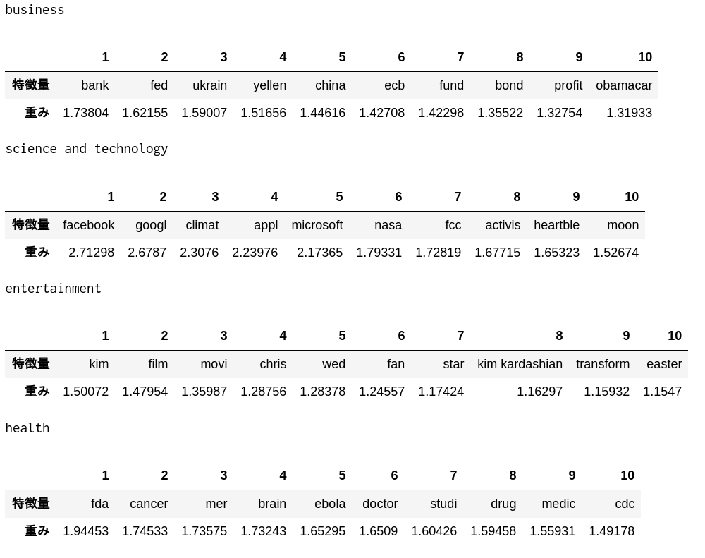
57. Confirmation of feature weights

Check the top 10 features with high weights and the top 10 features with low weights in the logistic regression model learned in> 52.

code

def show_weight(directional, N):
    for i, cat in enumerate(categories):
        indices = lr.coef_[i].argsort()[::directional][:N]
        best = np.array(features)[indices]
        weight = lr.coef_[i][indices]
        print(category_names[i])
        display(pd.DataFrame([best, weight], index = ['Feature value', 'weight'], columns = np.arange(N) + 1))

Top 10 features with large weight

code

show_weight(-1, 10)

code

show_weight(1, 10)

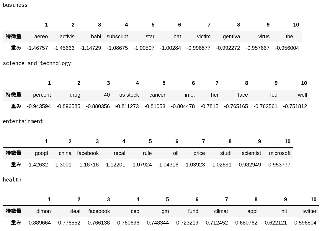
It seems that such features have been extracted.

58. Change regularization parameters

When training a logistic regression model, the degree of overfitting during learning can be controlled by adjusting the regularization parameters. Learn the logistic regression model with different regularization parameters and find the accuracy rate on the training data, validation data, and evaluation data. Summarize the results of the experiment in a graph with the regularization parameters on the horizontal axis and the accuracy rate on the vertical axis.

code

import matplotlib.pyplot as plt
import japanize_matplotlib
from tqdm import tqdm

Since it takes time, monitor with tqdm.tqdm.

code

Cs = np.arange(0.1, 5.1, 0.1)
lrs = [LogisticRegression(C=C, max_iter=1000).fit(train_x, train_t) for C in tqdm(Cs)]

code

train_accs = [accuracy(lr, train_x, train_t) for lr in lrs]
valid_accs = [accuracy(lr, valid_x, valid_t) for lr in lrs]
test_accs = [accuracy(lr, test_x, test_t) for lr in lrs]

code

plt.plot(Cs, train_accs, label = 'Learning')
plt.plot(Cs, valid_accs, label = 'Verification')
plt.plot(Cs, test_accs, label = 'Evaluation')
plt.legend()
plt.show()

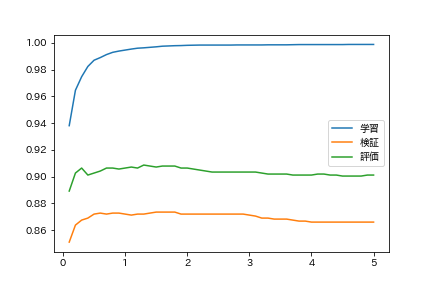
You are overfitting when regularization is weak.

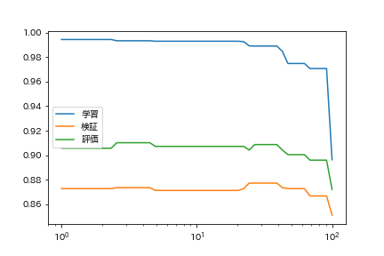
59. Searching for hyperparameters

Learn the categorization model while changing the learning algorithm and learning parameters. Find the learning algorithm / parameter that gives the highest accuracy rate on the evaluation data.

Let's change the censoring error.

code

tols = np.logspace(0, 2, 50)
lrs = [LogisticRegression(tol=tol, max_iter=1000).fit(train_x, train_t) for tol in tqdm(tols)]

code

train_accs = [accuracy(lr, train_x, train_t) for lr in lrs]
valid_accs = [accuracy(lr, valid_x, valid_t) for lr in lrs]
test_accs = [accuracy(lr, test_x, test_t) for lr in lrs]

code

plt.plot(tols, train_accs, label = 'Learning')
plt.plot(tols, valid_accs, label = 'Verification')
plt.plot(tols, test_accs, label = 'Evaluation')
plt.xscale('log')
plt.legend()
plt.show()

I would like to try other than logistic regression.

So, looking at sklearn's famous flowchart, I feel like something is wrong.

Naive bayes

code

from sklearn.naive_bayes import MultinomialNB

code

nb = MultinomialNB()
nb.fit(train_x, train_t)

output

MultinomialNB(alpha=1.0, class_prior=None, fit_prior=True)

code

accuracy(nb, train_x, train_t)

output

0.9429988768251591

code

accuracy(nb, test_x, test_t)

output

0.8907185628742516

Text classification COSPA strongest naive bayes

Linear support vector machine

code

from sklearn.svm import LinearSVC

code

svc = LinearSVC(C=0.1)
svc.fit(train_x,train_t)

output

LinearSVC(C=0.1, class_weight=None, dual=True, fit_intercept=True,
          intercept_scaling=1, loss='squared_hinge', max_iter=1000,
          multi_class='ovr', penalty='l2', random_state=None, tol=0.0001,
          verbose=0)

code

accuracy(svc, train_x, train_t)

output

0.9908274054661176

code

accuracy(svc, test_x, test_t)

output

0.9041916167664671

It's very good.

Next is Chapter 7

Language processing 100 knocks 2020 Chapter 7: Word vector