Learning Python with ChemTHEATER 02
Part 2 Statistical inference
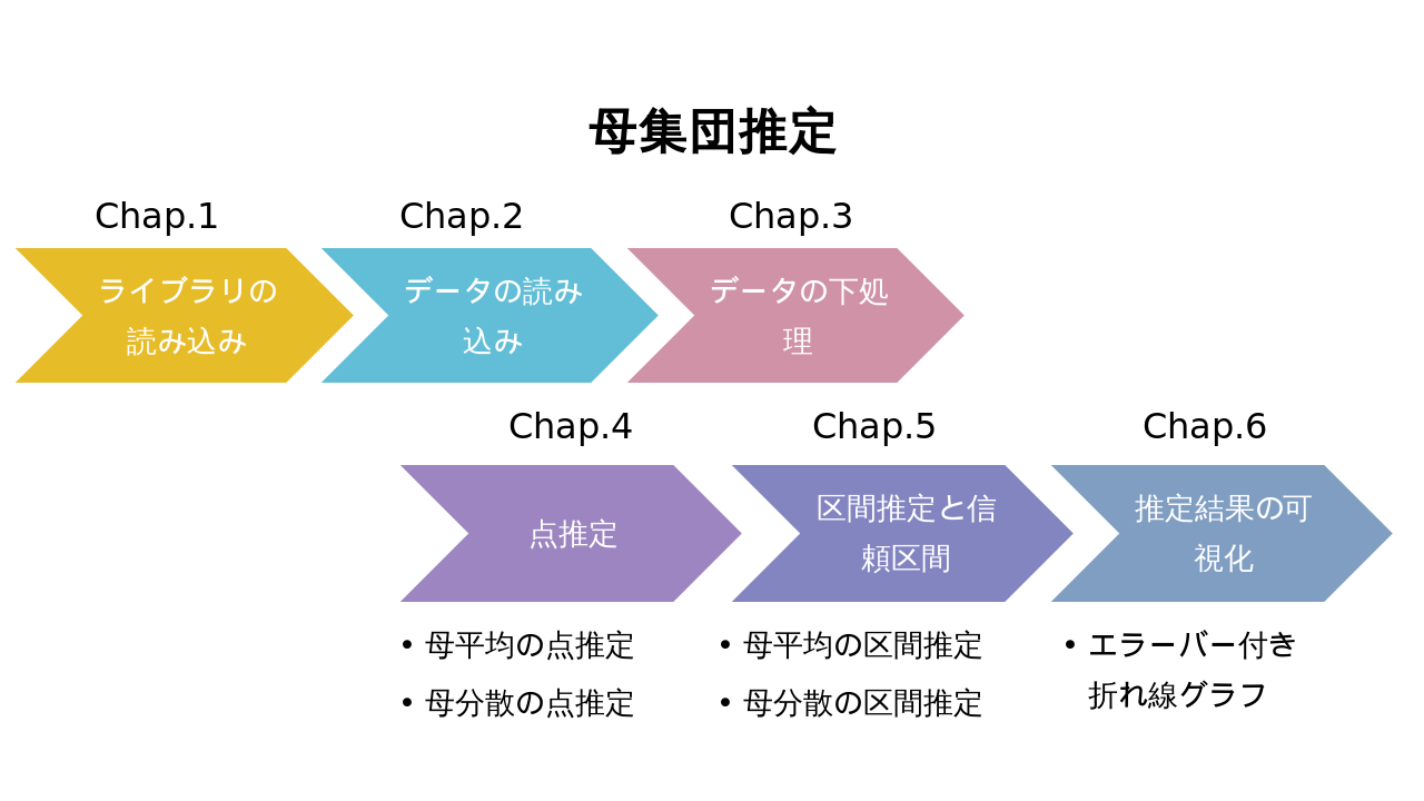
Chap.0 Overall flow
Part 2 makes statistical inferences. In the natural sciences, it is not possible to directly survey all the survey targets (nature), so sample surveys are common.
At that time, statistical inference is to estimate the distribution of the entire unknown population from the obtained sample (a part of the population).
Loading the Chap.1 library
%matplotlib inline
import numpy as np
from scipy import stats
import math
import pandas as pd
from matplotlib import pyplot as plt
First, start by loading the required libraries. The first line is a magic command to display matplotlib in Jupyter Notebook as in Part 1.
The second and subsequent lines are the libraries used this time. Of these libraries, the math library is built into Python as standard. Other libraries are installed in Anaconda.
By the way, math and Numpy are similar in function, but math is a function built into standard Python, and Numpy is an extension module that makes complex numerical calculations efficient, and their roles are different.
| Library | Overview | Purpose of use this time | Official URL |
|---|---|---|---|
| NumPy | Numerical calculation library | Used for numerical calculation in statistical processing | https://www.numpy.org |
| Scipy | Scientific Computational Library | Used for calculation of statistical inference | https://www.scipy.org |
| math | Standard Numerical Library | Used for simple calculations such as square roots | https://docs.python.org/ja/3/library/math.html |
| pandas | Data analysis library | Used for data reading and formatting | https://pandas.pydata.org |
| Matplotlib | Graph drawing library | Used for data visualization | https://matplotlib.org |
Reading Chap.2 data
This time, we will use the data of Skipjack ( Katsuwonus pelamis ). Refer to Chapter.4 of Part 0, and download the bonito sample data and measurement data from the Sample Search of ChemTHEATER.
Once downloaded, move the measured data and samples data to the folder containing this notebook file. After that, after restarting Anaconda, use the read_csv function of pandas as in Part 1 to read both the measurement data and the sample data.
data_file = "measureddata_20190930045953.tsv"    #Change the string entered in the variable to the tsv file name of your measured data
chem = pd.read_csv(data_file, delimiter="\t")
chem = chem.drop(["ProjectID", "ScientificName", "RegisterDate", "UpdateDate"], axis=1)    #Remove duplicate columns when joining with samples later

sample_file = "samples_20190930045950.tsv"    #Change the string entered in the variable to the tsv file name of your samples
sample = pd.read_csv(sample_file, delimiter="\t")
When reading or processing a file programmatically like python, it is better to make a habit of checking whether the file can be read as expected. By the way, in the case of Jupyter Notebook, if you enter only the variable name, the contents of that variable will be displayed in Out, which is convenient.
chem
| MeasuredID | SampleID | ChemicalID | ChemicalName | ExperimentID | MeasuredValue | AlternativeData | Unit | Remarks | |
|---|---|---|---|---|---|---|---|---|---|
| 0 | 1 | SAA000001 | CH0000096 | ΣPCBs | EXA000001 | 6.659795 | NaN | ng/g wet | NaN |
| 1 | 2 | SAA000002 | CH0000096 | ΣPCBs | EXA000001 | 9.778107 | NaN | ng/g wet | NaN |
| 2 | 3 | SAA000003 | CH0000096 | ΣPCBs | EXA000001 | 5.494933 | NaN | ng/g wet | NaN |
| 3 | 4 | SAA000004 | CH0000096 | ΣPCBs | EXA000001 | 7.354636 | NaN | ng/g wet | NaN |
| 4 | 5 | SAA000005 | CH0000096 | ΣPCBs | EXA000001 | 9.390950 | NaN | ng/g wet | NaN |
| ... | ... | ... | ... | ... | ... | ... | ... | ... | ... |
| 74 | 75 | SAA000082 | CH0000096 | ΣPCBs | EXA000001 | 3.321208 | NaN | ng/g wet | NaN |
| 75 | 76 | SAA000083 | CH0000096 | ΣPCBs | EXA000001 | 3.285111 | NaN | ng/g wet | NaN |
| 76 | 77 | SAA000084 | CH0000096 | ΣPCBs | EXA000001 | 0.454249 | NaN | ng/g wet | NaN |
| 77 | 78 | SAA000085 | CH0000096 | ΣPCBs | EXA000001 | 0.100000 | <1.00E-1 | ng/g wet | NaN |
| 78 | 79 | SAA000086 | CH0000096 | ΣPCBs | EXA000001 | 0.702224 | NaN | ng/g wet | NaN |
79 rows × 9 columns
sample
| ProjectID | SampleID | SampleType | TaxonomyID | UniqCodeType | UniqCode | SampleName | ScientificName | CommonName | CollectionYear | ... | |
|---|---|---|---|---|---|---|---|---|---|---|---|
| 0 | PRA000001 | SAA000001 | ST008 | 8226 | es-BANK | EF00564 | NaN | Katsuwonus pelamis | Skipjack tuna | 1998 | ... |
| 1 | PRA000001 | SAA000002 | ST008 | 8226 | es-BANK | EF00565 | NaN | Katsuwonus pelamis | Skipjack tuna | 1998 | ... |
| 2 | PRA000001 | SAA000003 | ST008 | 8226 | es-BANK | EF00566 | NaN | Katsuwonus pelamis | Skipjack tuna | 1998 | ... |
| 3 | PRA000001 | SAA000004 | ST008 | 8226 | es-BANK | EF00567 | NaN | Katsuwonus pelamis | Skipjack tuna | 1998 | ... |
| 4 | PRA000001 | SAA000005 | ST008 | 8226 | es-BANK | EF00568 | NaN | Katsuwonus pelamis | Skipjack tuna | 1998 | ... |
| ... | ... | ... | ... | ... | ... | ... | ... | ... | ... | ... | ... |
| 74 | PRA000001 | SAA000082 | ST008 | 8226 | es-BANK | EF00616 | NaN | Katsuwonus pelamis | Skipjack tuna | 1999 | ... |
| 75 | PRA000001 | SAA000083 | ST008 | 8226 | es-BANK | EF00617 | NaN | Katsuwonus pelamis | Skipjack tuna | 1999 | ... |
| 76 | PRA000001 | SAA000084 | ST008 | 8226 | es-BANK | EF00619 | NaN | Katsuwonus pelamis | Skipjack tuna | 1999 | ... |
| 77 | PRA000001 | SAA000085 | ST008 | 8226 | es-BANK | EF00620 | NaN | Katsuwonus pelamis | Skipjack tuna | 1999 | ... |
| 78 | PRA000001 | SAA000086 | ST008 | 8226 | es-BANK | EF00621 | NaN | Katsuwonus pelamis | Skipjack tuna | 1999 | ... |
79 rows × 66 columns
Chap.3 Data preparation
After reading the data, the next step is to prepare the data.
First, the data divided into two (chem and sample) are integrated, and only the necessary data is extracted. This time, we want to use the bonito ΣPCB data, so only the data whose "ChemicalName" column value is "ΣPCB" is extracted.
df = pd.merge(chem, sample, on="SampleID")
data = df[df["ChemicalName"] == "ΣPCBs"]
Next, check if the unit of measurement data is different. This is because if the unit of data is different as in Part 1, it is not possible to simply compare and integrate.
data["Unit"].unique()
array(['ng/g wet'], dtype=object)
You can use the
pandas unique method to see a list of the values contained in that dataframe. Here, if you output the list of values included in the "Unit" column, you can see that it is only "ng / g wet", so this time, it is not necessary to divide the data by unit. </ p>
Finally, the column with only N / A is deleted, and the data preparation is completed.
data = data.dropna(how='all', axis=1)
data
| MeasuredID | SampleID | ChemicalID | ChemicalName | ExperimentID | MeasuredValue | AlternativeData | Unit | ProjectID | SampleType | ... | |
|---|---|---|---|---|---|---|---|---|---|---|---|
| 0 | 1 | SAA000001 | CH0000096 | ΣPCBs | EXA000001 | 6.659795 | NaN | ng/g wet | PRA000001 | ST008 | ... |
| 1 | 2 | SAA000002 | CH0000096 | ΣPCBs | EXA000001 | 9.778107 | NaN | ng/g wet | PRA000001 | ST008 | ... |
| 2 | 3 | SAA000003 | CH0000096 | ΣPCBs | EXA000001 | 5.494933 | NaN | ng/g wet | PRA000001 | ST008 | ... |
| 3 | 4 | SAA000004 | CH0000096 | ΣPCBs | EXA000001 | 7.354636 | NaN | ng/g wet | PRA000001 | ST008 | ... |
| 4 | 5 | SAA000005 | CH0000096 | ΣPCBs | EXA000001 | 9.390950 | NaN | ng/g wet | PRA000001 | ST008 | ... |
| ... | ... | ... | ... | ... | ... | ... | ... | ... | ... | ... | ... |
| 74 | 75 | SAA000082 | CH0000096 | ΣPCBs | EXA000001 | 3.321208 | NaN | ng/g wet | PRA000001 | ST008 | ... |
| 75 | 76 | SAA000083 | CH0000096 | ΣPCBs | EXA000001 | 3.285111 | NaN | ng/g wet | PRA000001 | ST008 | ... |
| 76 | 77 | SAA000084 | CH0000096 | ΣPCBs | EXA000001 | 0.454249 | NaN | ng/g wet | PRA000001 | ST008 | ... |
| 77 | 78 | SAA000085 | CH0000096 | ΣPCBs | EXA000001 | 0.100000 | <1.00E-1 | ng/g wet | PRA000001 | ST008 | ... |
| 78 | 79 | SAA000086 | CH0000096 | ΣPCBs | EXA000001 | 0.702224 | NaN | ng/g wet | PRA000001 | ST008 | ... |
79 rows × 35 columns
Chap.4 point estimation
Of the statistical inferences that infer the population from a sample, point estimation is the pinpoint estimation. Here, we try to estimate the ΣPCB concentration of the population (whole individual in the collection area) from the ΣPCB concentration sample detected in skipjack.
First, in order to calculate year by year and see the transition of the change, check how many years the data is included.
data['CollectionYear'].unique()
array([1998, 1997, 1999, 2001], dtype=int64)
From the unique method above, it was found that the data set contains data for the three years 1997-1999 and 2001. First, let's take out the 1997 data. At this time, change the extracted data to Numpy's ndarray 1 format so that future calculations will be easier.
Similarly, the data for 1998 and 1999 are also extracted.
Here, the unbiased estimators of mean and variance are calculated. Similarly, calculate the unbiased estimator of the variance. The Numpy var function can calculate either variance, and the unbiased variance is output with the parameter ddof = 1. However, note that the sample variance of ddof = 0 is output by default. Similarly, calculate the unbiased estimators of the mean and variance for 1998 and 1999.
Here, the obtained representative values are summarized. First,
In Chap.5, unlike the point estimation obtained in Chap.4, interval estimation is performed to estimate the population mean and population variance within a statistically constant range.
First, before estimating the interval, check the number of data in each year's dataset. The number of data can be calculated by using the len function implemented as standard in python.
From the above, the total number of data in the data set for each year from 1997 to 1999 is known.
Of these, the 1997 dataset is a large sample of $ n = 50 $, and the 1998 and 1999 datasets are $ n = \ left \ {\ begin {array} {ll}, respectively. 15 & \ left (1998 \ right) \\ 13 & \ left (1999 \ right) \ end {array} \ right. $, Which is a small sample. First, the interval of the population mean is estimated from the 1997 data set. In this case, since the population variance is unknown and the sample is large ($ n> 30 $), the sample mean ($ \ overline X $) is normally distributed $ N \ left (\ mu, \ frac {s ^ 2} { n} \ right) $ can be approximated. Therefore, if the population mean is estimated by the confidence interval ($ \ alpha $), the confidence interval is as shown in the following equation.
$\overline X - z_\frac{\alpha}{2} \sqrt{\frac{s^2}{n}} < \mu < \overline X - z_\frac{\alpha}{2} \sqrt{\frac{s^2}{n}} $
In python, if you use Scipy's stas.norm.interval (), you can get the range of alpha × 100% in the normal distribution of mean (loc) and standard deviation (scale) centered on the median. Next, we estimate the interval of the population mean for the 1998 and 1999 datasets. These are small samples ($ n \ leq 30 $) with unknown population variance. In this case, the population mean $ \ mu $ is not the normal distribution $ N \ left (\ mu, \ frac {s ^ 2} {n} \ right) $, but the t distribution with degrees of freedom ($ n-1 $). To use. Therefore, if the population mean is estimated by the confidence interval ($ \ alpha $), the confidence interval is as shown in the following equation.
$\overline X - t_\frac{\alpha}{2}\left(n-1\right)\sqrt{\frac{s^2}{n}} < \mu < \overline X + t_\frac{\alpha}{2}\left(n-1\right)\sqrt{\frac{s^2}{n}} $
In python, if you use stats.t.interval (), the range where the t distribution of mean (loc), standard deviation (scale), and degrees of freedom (df) is alpha × 100% is centered on the median. Can be obtained as. The 95% confidence interval means that the population mean is within that range with a 95% probability. That is, if the reliability ($ \ alpha $) is reduced, the probability that the population mean is included in the confidence interval is reduced, and at the same time, the confidence interval is narrowed.
Next, the interval estimation of the population variance is performed. In the interval estimation of the population variance ($ \ sigma ^ 2 $), $ \ frac {\ left (n-1 \ right) s ^ 2} {\ sigma ^ 2} $ has $ (n-1) $ degrees of freedom. Use to follow the $ \ chi ^ 2 $ distribution of.
$\chi_\frac{\alpha}{2}\left(n-1\right) \leq \frac{\left( n-1 \right)s^2}{\sigma^2} \leq \chi_{1-\frac{\alpha}{2}}\left(n-1\right)$
First, the percentage points of the $ \ chi ^ 2 $ distribution of degrees of freedom ($ n-1 $) ($ \ chi_ \ frac {\ alpha} {2} \ left (n-1 \ right), \ chi_ Find {1- \ frac {\ alpha} {2}} \ left (n-1 \ right) $). Here, the reliability is 0.95. Next, find the confidence interval. For derivation, refer to the following formula.
$\frac{\left(n-1\right)s^2}{\chi_\frac{\alpha}{2}\left(n-1\right)} \leq \sigma^2 \leq \frac{\left(n-1\right)s^2}{\chi_{1-\frac{\alpha}{2}}\left(n-1\right)}$
Similarly, for the 1998 and 1999 datasets, the variance interval is estimated. Note that unlike the interval estimation of the population mean, the distribution of $ \ frac {\ left (n-1 \ right) s ^ 2} {\ sigma ^ 2} $ is $ \ chi ^ 2 regardless of the sample size. Follow the $ distribution.
Now, let's visualize the population mean estimated in Chap.4 and Chap.5 on a graph.
First, the values of the population means estimated by points in Chap.4 are summarized in chronological order.
Next, the confidence intervals of the population mean with a reliability of 95% estimated in Chap.5 are also summarized in chronological order.
The 95% confidence interval of the population mean cannot be used for visualization as it is, so the width of the confidence interval is calculated.
Finally, visualize with matplotlib. Confidence intervals are displayed with error bars. When displaying the error bar with matplotlib, use the errorbar method. 1 A data format for storing n-th order matrices in Numpy.
Recommended Posts
pcb_1997 = np.array(data[data['CollectionYear']==1997]["MeasuredValue"]) #Extract only 1997 measurements
pcb_1997
array([ 10.72603788,   9.22208078,   7.59790835,  30.95079465,
        15.27462553,  14.15719633,  13.28955903,  14.87712806,
         9.86650189,  18.26554514,   3.39951845,   6.58172781,
        12.43564814,   6.1948639 ,   6.41605666,   4.98827291,
        12.36669815,  31.17955551,   8.16184346,   4.60893266,
        36.85826409,  52.99841724,  39.22500351,  53.92302702,
        69.4308048 ,  73.97686479, 125.3887794 ,  45.39974771,
        54.12726127,  39.77794045, 101.2736126 ,  38.06220403,
       126.8301693 ,  70.25308435,  31.24246301,  21.3958656 ,
        41.85726522,  30.91112132,  81.12597135,  10.76755148,
        24.20442213,  24.57497594,  14.84353549,  59.53687389,
        52.78443082,   8.4644697 ,   4.15293758,   3.31957452,
         4.51832675,   6.98373973])
pcb_1998 = np.array(data[data['CollectionYear']==1998]["MeasuredValue"]) #Extract only 1998 measurements
pcb_1999 = np.array(data[data['CollectionYear']==1999]["MeasuredValue"]) #Extract only 1999 measurements
First, the unbiased estimator of the mean ($ \ hat {\ mu} $), which takes advantage of the fact that the expected value of the sample mean ($ \ overline {X} $) is equal to the population mean. (See formula below)
$$ E \left(\overline X \right) = E\left(\frac{1}{n} \sum_{i=1}^{n} \left(x_i\right)\right) = \frac{1}{n}\sum_{i=1}^{n} E\left(x_i\right) = \frac{1}{n} \times n\mu = \mu \\ \therefore \hat\mu = \overline{x} $$s_mean_1997 = np.mean(pcb_1997)
s_mean_1997
31.775384007760003
At this time, the expected value of the sample variance ($ S ^ 2 $) does not take the same value as the population variance ($ \ sigma ^ 2 $), and it is necessary to obtain the unbiased variance ($ s ^ 2 $) instead. Pay attention to.
$$\hat\sigma^2 \neq S^2 = \frac{1}{n} \sum_{i=1}^{n} \left( x_i - \overline X \right) \\ \hat\sigma^2 = s^2 = \frac{1}{n-1} \sum_{i=1}^{n} \left( x_i - \overline X \right)$$
$$\mathrm{np.var}\left(x_1 \ldots x_n, \mathrm{ddof=0}\right): S^2 = \frac{1}{n} \sum_{i=1}^{n} \left( x_i - \overline X \right) \\
\mathrm{np.var}\left(x_1 \ldots x_n, \mathrm{ddof=1}\right): \hat\sigma^2 = \frac{1}{n-1} \sum_{i=1}^{n} \left( x_i - \overline X \right)$$u_var_1997 = np.var(pcb_1997, ddof=1)
u_var_1997
942.8421749786518
s_mean_1998, s_mean_1999 = np.mean(pcb_1998), np.mean(pcb_1999)
u_var_1998, u_var_1999 = np.var(pcb_1998, ddof=1), np.var(pcb_1999, ddof=1)
s_mean_1997, s_mean_1998, s_mean_1999
(31.775384007760003, 17.493267312533337, 30.583242522000003)
u_var_1997, u_var_1998, u_var_1999
(942.8421749786518, 240.2211176248311, 1386.7753819003349)
Chap.5 Interval estimation and confidence interval
Sec.5-1 Interval estimation of population mean
n_1997 = len(pcb_1997)
n_1997
50
n_1998, n_1999 = len(pcb_1998), len(pcb_1999)
n_1998, n_1999
(15, 13)
Therefore, it should be noted that the subsequent interval estimation process is slightly different.
Here, the confidence interval is calculated with the reliability ($ \ alpha = 0.95 $).
m_interval_1997 = stats.norm.interval(alpha=0.95, loc=s_mean_1997, scale=math.sqrt(pcb_1997.var(ddof=1)/n_1997))
m_interval_1997
(23.26434483549182, 40.28642318002819)
Here, the confidence interval is calculated based on the reliability ($ \ alpha = 0.95 $).
m_interval_1998 = stats.t.interval(alpha=0.95, df=n_1998-1, loc=s_mean_1998, scale=math.sqrt(pcb_1998.var(ddof=1)/n_1998))
m_interval_1999 = stats.t.interval(alpha=0.95, df=n_1999-1, loc=s_mean_1999, scale=math.sqrt(pcb_1999.var(ddof=1)/n_1999))
m_interval_1997, m_interval_1998, m_interval_1999
((23.26434483549182, 40.28642318002819),
 (8.910169386248537, 26.076365238818138),
 (8.079678286109523, 53.086806757890486))
stats.norm.interval(alpha=0.9, loc=s_mean_1997, scale=math.sqrt(pcb_1997.var(ddof=1)/n_1997))
(24.63269477364296, 38.91807324187704)
Sec.5-2 Interval estimation of population variance
In python, Scipy's stats.chi2.interval () can be used to get the range of alpha x 100% of degrees of freedom (df).
chi_025_1997, chi_975_1997 = stats.chi2.interval(alpha=0.95, df=n_1997-1)
chi_025_1997, chi_975_1997
(31.554916462667137, 70.22241356643451)
v_interval_1997 = (n_1997 - 1)*np.var(pcb_1997, ddof=1) / chi_975_1997, (n_1997 - 1)*np.var(pcb_1997, ddof=1) / chi_025_1997
v_interval_1997
(657.8991553778869, 1464.0909168183869)
chi_025_1998, chi_975_1998 = stats.chi2.interval(alpha=0.95, df=n_1998-1)
chi_025_1999, chi_975_1999 = stats.chi2.interval(alpha=0.95, df=n_1999-1)
v_interval_1998 = (n_1998 - 1)*np.var(pcb_1998, ddof=1) / chi_975_1998, (n_1998 - 1)*np.var(pcb_1998, ddof=1) / chi_025_1998
v_interval_1999 = (n_1999 - 1)*np.var(pcb_1999, ddof=1) / chi_975_1999, (n_1999 - 1)*np.var(pcb_1999, ddof=1) / chi_025_1999
v_interval_1997, v_interval_1998, v_interval_1999
((657.8991553778869, 1464.0909168183869),
 (128.76076176378118, 597.4878836139195),
 (713.0969734866349, 3778.8609867211235))
chi_025_1997, chi_975_1997 = stats.chi2.interval(alpha=0.9, df=n_1997-1)
(n_1997 - 1)*np.var(pcb_1997, ddof=1) / chi_975_1997, (n_1997 - 1)*np.var(pcb_1997, ddof=1) / chi_025_1997
(696.4155490924242, 1361.5929987004467)
Chap.6 Visualization of estimation results
x_list = [1997, 1998, 1999]
y_list = [s_mean_1997, s_mean_1998, s_mean_1999]
interval_list = []
interval_list.append(m_interval_1997)
interval_list.append(m_interval_1998)
interval_list.append(m_interval_1999)
interval_list
[(23.26434483549182, 40.28642318002819),
 (8.910169386248537, 26.076365238818138),
 (8.079678286109523, 53.086806757890486)]
interval_list = np.array(interval_list).T[1] - y_list
x_list, y_list, interval_list
([1997, 1998, 1999],
 [31.775384007760003, 17.493267312533337, 30.583242522000003],
 array([ 8.51103917,  8.58309793, 22.50356424]))
This method specifies the X-axis value (here year), the Y-axis value (here the population mean of the point estimate), and the length of the error bar (here the width of the confidence interval).
fig = plt.figure()
ax = fig.add_subplot(1,1,1)
ax.errorbar(x=x_list, y=y_list, yerr=interval_list, fmt='o-', capsize=4, ecolor='red')
plt.xticks(x_list)
ax.set_title("Katsuwonus pelamis")
ax.set_ylabel("ΣPCBs [ng/g wet]")
plt.show()

footnote