Introduction

Do you guys do reinforcement learning? Reinforcement learning is a fun technology that can be applied to robots, games such as Go and Shogi, and dialogue systems.

Reinforcement learning is a learning control framework that adapts to the environment through trial and error. In supervised learning, the correct output was given to the input for learning. In reinforcement learning, instead of giving the correct output for the input, a scalar evaluation value called "reward" that evaluates the good or bad of a series of actions is given, and learning is performed using this as a clue. The framework of reinforcement learning is shown below.

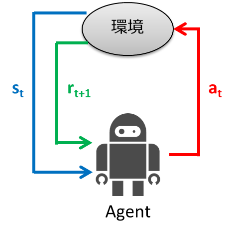
The agent observes the environment state $ s_t $ at time $ t $
Determine the action $ a_t $ from the observed state
Agent takes action
Environment transitions to new state $ s_ {t + 1} $
Earn $ r_ {t + 1} $ as a reward according to the transition
Learn
Repeat from step 1

The purpose of reinforcement learning is to obtain a state-to-behavior mapping (policy) that maximizes the gain (cumulative reward) that an agent obtains.

In reinforcement learning, the above framework is modeled by Markov decision processes (MDP), and learning algorithms are considered. In this article, we will explain reinforcement learning separately in theory and practice. In the theory section, we will explain MDP and learning algorithms, and in the practice section, we will implement what was explained in the theory section using the programming language Python. We recommend that you read them in order, but if you say "Komake Kota is good!", Skip the theory section and read the practice section.

Theory

First, I will explain the theory of reinforcement learning with examples. Here, after explaining the problem setting of the example, we will explain the Markov decision process. Now that you understand the Markov decision process, I will explain how to learn it.

Problem setting

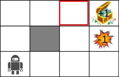
Now, in explaining MDP, consider the following maze world.

The rules of the maze world are as follows.

Agent is in a grid
Agent cannot cross the wall (gray)
Agents may not always work the way they want
80% chance to move correctly, 10% chance to move to the left in the direction you intended to move, and 10% chance to move to the right
If there is a wall where you want to move, stay there
Agent receives reward at each time
When you reach the goal (treasure chest) or trap (explosion), the game ends and you return to the start position.

The stochastic transition will be explained in a little more detail using the figure below.

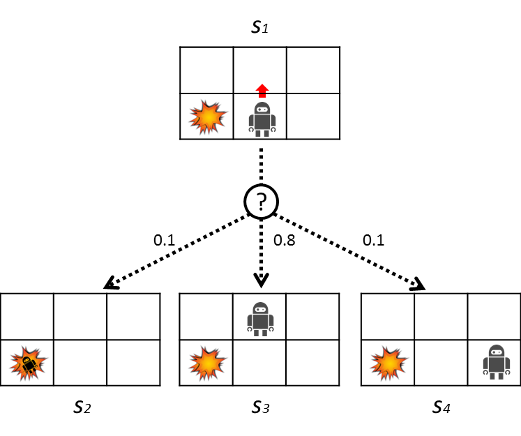
Here the robot is trying to move up. At this time, there is an 80% chance of moving up, but a 10% chance of moving to the left and the remaining 10% of moving to the right. The transition probabilities are shown in the table below.

s'	P(s' \mid s_1, a)
s_2	0.1
s_3	0.8
s_4	0.1

Markov decision processes (MDP)

Now, did you understand the problem setting? Now that we know, we will model the problem with MDP.

MDP is defined by the following 4-term set

M = (S, A, T, R)

What is each?

State set: $ s \ in S $
Action set: $ a \ in A $
Transition function: $ T (s, a, s') \ sim P (s' \ mid s, a) $
Reward function: $ R (s) $, $ R (s, a) $, $ R (s, a, s') $

Let's apply each to the problem settings explained above.

The state set represents the set of states that the environment can take, and in the case of the example, it represents all the cells of the grid.
An action set is a type of action that an agent can take. In the case of the example, there are four types of agents because they can move up, down, left, and right.
The transition function represents the probability of transitioning to the next state $ s'$ when the action $ a $ is taken in one state $ s $. As explained in the figure above.
Reward is the value received from the environment as a result of a new transition that determines the action to be taken from the observed state. I will explain in detail later.

The purpose of this MDP is to learn behavioral strategies that maximize gain (= cumulative reward). This action strategy is called ** policy **.

A little more about policy

The goal of MDP is to get the best policy $ \ pi ^ *: S \ rightarrow A $. Policy can be thought of as a function that maps state to action. Policies tell us what to do in each situation. Optimal policies also maximize expected gains.

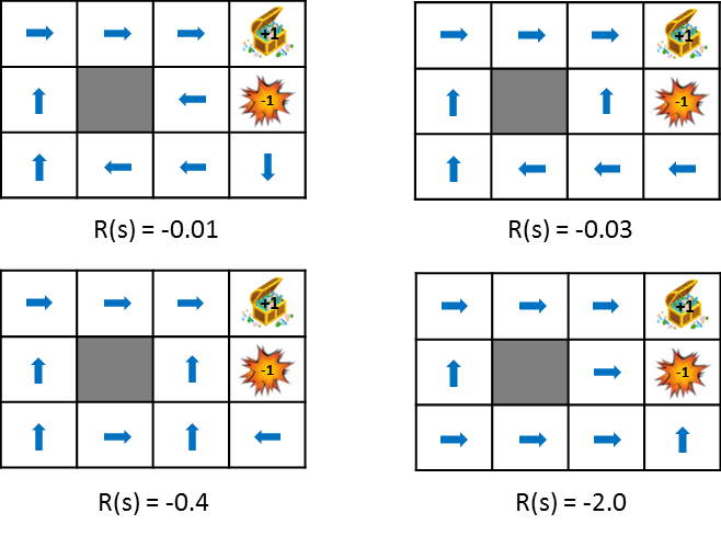
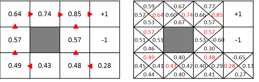
Let's take a look at the optimal policy changes when changing the rewards obtained during the transition. This figure shows the change in policy when the reward obtained from the state transition is gradually reduced (penalty is increased). Policy learns from the idea of maximizing the expected gains obtained. Therefore, if the penalty due to the state transition is small, it will try to aim for the goal even if it detours, and if the penalty is large, it will take a strategy to end the game promptly. Still images are also available for easy comparison.

A little more about rewards

So far, I have said that I will maximize cumulative rewards in order to learn policy. Since you can get the reward $ R (s_t) $ at each time, the cumulative reward can be expressed as:

\begin{align}
U([s_0, s_1, s_2,\ldots]) &= R(s_0) + R(s_1) + R(s_2) + \cdots \\
    &= \sum_{t=0}^{\infty}R(s_t)
\end{align}

You can use this simple cumulative reward, but for some reason you can discount future rewards with the discount factor $ \ gamma (0 \ leq \ gamma <1) $ as shown in the formula below. Cumulative rewards are used. This will give you more weight on your current rewards than on your future rewards.

\begin{align}
U([s_0, s_1, s_2,\ldots]) &= R(s_0) + \gamma R(s_1) + \gamma^2 R(s_2) + \cdots \\
    &= \sum_{t=0}^{\infty}\gamma^t R(s_t)
\end{align}

The reasons for using such discount rewards are as follows.

The value does not diverge computationally
In a real environment, it is not reasonable to consider all time series rewards with the same weight, as the environment can change over time.

How to find the best policy

So far, we know about the model called MDP. The remaining question is how to find the best policy. In the following, we will explain the value iterative method and Q-Learning as algorithms for finding the optimal policy.

Value Iteration

The value iterative method calculates the expected gain from the state $ s $ when the optimal action is continued. The expected value of the gain obtained is considered because of the stochastic transition.

Once we know this expected gain, we know the value we will get in the future from our current state of $ s $, and we should be able to choose actions that maximize that value. The value is calculated by the following state value function. It looks complicated, but in short, it's just calculating the (expected) discount cumulative reward.

U(s) = R(s) + \gamma \max_a\sum_{s'} P(s' \mid s,a) U(s')

There is a non-linear calculation called max in this equation, and it is difficult to solve it with a matrix or the like. Therefore, iterative calculations are performed to gradually update the value. This is the reason for the name of the value iteration method. The value iterative algorithm is shown below. The amount of calculation isO(|S|^2 |A|)is.

Initialize $ U (s) $ to an appropriate value (such as zero) for all states $ s $

Calculate the following formula for all $ U (s) $ and update the values

U(s) \leftarrow R(s) + \gamma \max_a\sum_{s'} P(s' \mid s,a) U(s')

 > 3. Repeat step 2 until the values converge

 There is a part to calculate max in the above formula, but it is necessary to record the action a whose value is the maximum value. Therefore, there is a problem that it is difficult to understand the optimal policy (behavior) only with $ U (s) $. Therefore, the following Q function is introduced. Also called the action value function.

```math
Q^*(s,a) = R(s) + \gamma \sum_{s'} P(s' \mid s,a) \max_{a'}Q^*(s', a')

** $ Q ^ * (s, a) $ ** represents the expected value of the discounted cumulative reward if you continue to take the optimal policy after selecting action a in ** state $ s $. There is a difference between $ U (s) $ and $ Q ^ * (s, a) $ whether they hold only the maximum value in each state or the value for each action. Therefore, the maximum Q value in the state s is equal to $ U (s) $, and the action a with this Q value is the optimal action. The figure below is the image.

The value iterative method when using the Q function is as follows.

Initialize $ Q ^ * (s, a) $ to an appropriate value (such as zero) for all states $ s $

Calculate the following formula and update the value for all $ Q ^ * (s, a) $

Q^(s,a) \leftarrow R(s) + \gamma \sum_{s'} P(s' \mid s,a) \max_{a'}Q^(s', a')


 > 3. Repeat step 2 until the values converge


 At this point it's easy to find the best policy $ \ pi ^ * (s) $. It is calculated below.

```math
\pi^*(s) = arg\max_{a}Q^*(s,a)

Calculation example

Since it's a big deal, let's try to calculate the value of the red place below. Use the following formula for the calculation.

U(s) \leftarrow R(s) + \gamma \max_a\sum_{s'} P(s' \mid s,a) U(s')

$ \ Gamma = 0.5 $, $ R (s) = -0.04 $, the transition probability is 0.8 in the direction you want to go, and 0.1 on each side.

Under the above conditions, the value in the red area is ...

\begin{align}
U(s) &= -0.04 + 0.5 \cdot (0.8 \cdot 1 + 0.1 \cdot 0 + 0.1 \cdot 0)\\
&= -0.04 + 0.4\\
&= 0.36
\end{align}

Is required.

Q-Learning Now, I am relieved that the optimal policy is required by the value iteration method. That's not the wholesaler. What's wrong?

Until now, we knew about state transition probabilities. However, considering the actual problem, it is rare that the state transition probability is known. Imagine chess or shogi. Is the probability of transition from one board (state) to another (other state) given in advance? You haven't been given it, right? In such cases, the value iteration method cannot be used.

That is where Q-Learning, which can be said to be a reinforcement learning version of the value iteration method, comes out. In Q-Learning Calculate the estimated $ \ hat {Q} ^ {\ *} (s_t, a_t) $ for $ \ hat {Q} ^ {\ *} (s, a) $. By using Q-Learning, you can learn the optimal policy even in situations where you do not know the transition probability. The Q-Learning algorithm is as follows.

Initialize $ \ hat Q ^ * (s_t, a_t) $ with an appropriate value

Updated the action value estimate using the following formula. However, $ \ alpha $ is the learning rate of $ 0 \ leq \ alpha \ leq 1 $.

\hat Q^(s_t, a_t) \leftarrow \hat Q^(s_t, a_t) + \alpha \Bigl[ r_{t+1} + \gamma \max_{a \in A}\hat Q^(s_{t+1}, a) - \hat Q^(s_t, a_t) \Bigr]

 > 3. Advance time step $ t $ to $ t + 1 $ and back to 2

 You can get the optimal $ Q ^ * (s, a) $ by repeating this calculation.

<!--
 Comparing the update formula of the value iteration method (Q function version) and the update formula of Q-Learning, the transition probability $ P (s'\ mid s, a) $ is calculated for the Q function in the value iteration method. Although it is used, it is not used because it is unknown in the situation where Q-Learning is used. By performing iterative calculations
-->

# Practical edition
 Let's see what happens if we do what we explained above in Python.

## Value iterative method
 First is the value iteration method.
 The value iteration method is based on the clean code (mdp.py) in [UC Berkeley](https://github.com/aimacode/aima-python).

### MDP class
 First, from MDP, which is the base class. Inherit this and create a GridMDP class.

```python
class MDP:

    def __init__(self, init, actlist, terminals, gamma=.9):
        self.init = init
        self.actlist = actlist
        self.terminals = terminals
        if not (0 <= gamma < 1):
            raise ValueError("An MDP must have 0 <= gamma < 1")
        self.gamma = gamma
        self.states = set()
        self.reward = {}

    def R(self, state):
	return self.reward[state]

    def T(self, state, action):
        raise NotImplementedError

    def actions(self, state):
        if state in self.terminals:
            return [None]
        else:
            return self.actlist

The \ _ \ _ init \ _ \ _ method receives the following parameters:

init: Initial state.
actlist: Actions that can be taken in each state.
terminals: list of terminated states
gamma: Discount factor

The ** R ** method returns the reward for each state. The ** T ** method is a transition model. Although it is an abstract method here, it returns a list of transition probabilities to the next state and tuples (probability, s') of the next state when the action $ a $ is taken in the state $ s $. We will implement it with Grid MDP. The ** actions ** method returns a list of actions that can be taken in each state.

GridMDP class

The GridMDP class is a concrete class of the base class MDP. This class is for expressing the world of the maze explained in the example.

class GridMDP(MDP):

    def __init__(self, grid, terminals, init=(0, 0), gamma=.9):
        grid.reverse()  # because we want row 0 on bottom, not on top                                                                                                  
        MDP.__init__(self, init, actlist=orientations,
                     terminals=terminals, gamma=gamma)
        self.grid = grid
        self.rows = len(grid)
        self.cols = len(grid[0])
        for x in range(self.cols):
            for y in range(self.rows):
                self.reward[x, y] = grid[y][x]
                if grid[y][x] is not None:
                    self.states.add((x, y))

    def T(self, state, action):
        if action is None:
            return [(0.0, state)]
        else:
            return [(0.8, self.go(state, action)),
                    (0.1, self.go(state, turn_right(action))),
                    (0.1, self.go(state, turn_left(action)))]

    def go(self, state, direction):
        state1 = vector_add(state, direction)
        return state1 if state1 in self.states else state

    def to_grid(self, mapping):
        return list(reversed([[mapping.get((x, y), None)
                               for x in range(self.cols)]
                              for y in range(self.rows)]))

    def to_arrows(self, policy):
        chars = {(1, 0): '>', (0, 1): '^', (-1, 0): '<', (0, -1): 'v', None: '.'}
        return self.to_grid({s: chars[a] for (s, a) in policy.items()})

The \ _ \ _ init \ _ \ _ method receives almost the same arguments as the MDP class, except that it receives the grid argument. The grid stores rewards for each state. Pass it like the following. None represents a wall.

GridMDP([[-0.04, -0.04, -0.04, +1],
        [-0.04, None,  -0.04, -1],
        [-0.04, -0.04, -0.04, -0.04]],
        terminals=[(3, 2), (3, 1)])

The ** go ** method returns the state when moving in the specified direction. The ** T ** method is as described in MDP. It's actually implemented here. The ** to_grid ** and ** to_arrows ** methods are display methods.

Implementation of value iterative method

def value_iteration(mdp, epsilon=0.001):
    U1 = {s: 0 for s in mdp.states}
    R, T, gamma = mdp.R, mdp.T, mdp.gamma
    while True:
        U = U1.copy()
        delta = 0
        for s in mdp.states:
            U1[s] = R(s) + gamma * max([sum([p * U[s1] for (p, s1) in T(s, a)])
                                        for a in mdp.actions(s)])
            delta = max(delta, abs(U1[s] - U[s]))
        if delta < epsilon * (1 - gamma) / gamma:
            return U


def best_policy(mdp, U):
    pi = {}
    for s in mdp.states:
        pi[s] = argmax(mdp.actions(s), key=lambda a: expected_utility(a, s, U, mdp))
    return pi


def expected_utility(a, s, U, mdp):
    return sum([p * U[s1] for (p, s1) in mdp.T(s, a)])

The ** value_iteration ** function takes an instance of GridMDP as input and a small value epsilon and returns U (s) in each state as output. It looks like the following.

>> value_iteration(sequential_decision_environment)
{(0, 0): 0.2962883154554812,
 (0, 1): 0.3984432178350045,
 (0, 2): 0.5093943765842497,
 (1, 0): 0.25386699846479516,
 (1, 2): 0.649585681261095,
 (2, 0): 0.3447542300124158,
 (2, 1): 0.48644001739269643,
 (2, 2): 0.7953620878466678,
 (3, 0): 0.12987274656746342,
 (3, 1): -1.0,
 (3, 2): 1.0}

Then, by passing the result calculated by the value_iteration function to the ** best_policy ** function, the optimum policy is obtained.

Run

Below is the code to try. However, as it is, it does not work because some required modules have not been imported. Therefore, if you want to actually run it, clone the repository here and run it.

sequential_decision_environment = GridMDP([[-0.04, -0.04, -0.04, +1],
                                           [-0.04, None,  -0.04, -1],
                                           [-0.04, -0.04, -0.04, -0.04]],
                                          terminals=[(3, 2), (3, 1)])

pi = best_policy(sequential_decision_environment, value_iteration(sequential_decision_environment, .01))

print_table(sequential_decision_environment.to_arrows(pi))

As a result of implementation, the following policies can be obtained.

>   >      >   .
^   None   ^   .
^   >      ^   <

Q-Learning There is no dent, it's just like a spring

Please write Q-Learning when you have physical strength.

Reference material

Udacity lecture video. The letters are hard to read, but the story is easy to understand.

Machine Learning: Reinforcement Learning

Japanese materials

English materials

Materials that explain Value Iteration in an easy-to-understand manner with figures

Reference materials when implementing Value Iteration

The mathematical expansion of the value function is polite

Reinforcement Learning Searching for optimal policies I:Bellman equations and optimal policies

Reinforcement learning starting with Python