Generate fake table data with GAN
Overview
Try CTGAN, one of the GANs for table data, against the Census Income dataset to generate fake table data. Train XGBoost with the generated data and verify how accurate it is compared to the original data.
CTGAN GAN is famous as a technology that can generate realistic fake images, but research on GAN for non-image data is also progressing. The following are the codes published in GAN corresponding to table data.
- MedGAN [arXiv:1703.06490][GitHub]
- TableGAN [arXiv:1806.03384][GitHub]
- TGAN [arXiv:1811.11264][GitHub]
- CTGAN [arXiv:1907.00503][GitHub]
As the name suggests, MedGAN is a model developed with medical data in mind and supports only categorical data. (There is also a model for medical images with the same name.) TableGAN and TGAN are models developed independently at the same time, and both support tables that contain both categorical and numerical data. In Japanese articles
-Increase titanic data with GAN (TGAN) for table data
TGAN is introduced in. This time, I will try CTGAN (Conditional Tabular GAN), which is an updated version of TGAN.
CTGAN is easy to install with pip.
pip install ctgan
Data preparation
Use a dataset called Census Income as the table data. This dataset is used to predict whether your annual income will exceed $ 50,000 from personal information such as gender, age, educational background and race. The data can be downloaded from the link above, but since it is included in CTGAN as demo data, it can be read as follows.
import numpy as np
import pandas as pd

from ctgan import load_demo
df0 = load_demo()
print(df0.shape)
# (32561, 15)
For some reason, the data read in this way contains a half-width space at the beginning of the category item. It doesn't matter if a half-width space is included in the amount to be sent to CTGAN and XGBoost, but it will be an obstacle when analyzing data, so remove it for the time being.
for col in df0.select_dtypes(exclude=np.number).columns:
    df0[col] = df0[col].str.replace(' ', '')
The first few lines are displayed as follows.
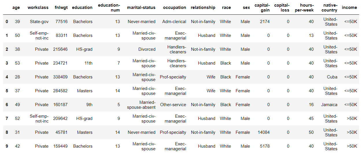 You can see that it consists of a categorical variable column and an integer column.
Of these columns, the following are excluded.
'fnlwgt': Seems like an ID number
'education-num': One-to-one correspondence with'education'
'capital-gain': Most lines contain 0s
'capital-loss': Same as above
You can see that it consists of a categorical variable column and an integer column.
Of these columns, the following are excluded.
'fnlwgt': Seems like an ID number
'education-num': One-to-one correspondence with'education'
'capital-gain': Most lines contain 0s
'capital-loss': Same as above
df0.drop(['fnlwgt', 'education-num', 'capital-gain', 'capital-loss'],
         axis=1, inplace=True)
By the way, this dataset does not contain missing values, and there is a'?' In the place where it seems to have been a missing value. This time, leave the'?'As it is and continue processing.
Then separate the dataset for training and testing. The training data will be used for both CTGAN training and XGBoost training.
df0_train, df_test = train_test_split(df0,
                                      test_size=0.2,
                                      random_state=0,
                                      stratify=df0['income'])
print(len(df0_train)) # 26048
print(len(df_test)) # 6513
Prepare another small training data.
df1_train, _ = train_test_split(df0_train,
                                test_size=0.9,
                                random_state=0,
                                stratify=df0_train['income'])
print(len(df1_train)) # 2604
Data generation
First, let's train CTGAN using the larger training data df0_train. When training, it is necessary to specify the column name of the categorical variable.
discrete_columns = [
    'workclass',
    'education',
    'marital-status',
    'occupation',
    'relationship',
    'race',
    'sex',
    'native-country',
    'income'
]
Learning can be done easily as follows. The input data corresponds to pandas.DataFrame and numpy.ndarray.
from ctgan import CTGANSynthesizer

ctgan0 = CTGANSynthesizer()
ctgan0.fit(df0_train, discrete_columns)
Learning runs 300 epoch with the default settings.
Generate data when training is complete. The generated data will be in the same format as the input data, so in this case pandas.DataFrame will be returned. The number of samples (number of rows) of data to be generated can be set freely. No matter how much you make it, it's free, so let's take the plunge and make 1 million lines.
n_samples = 1000000
df0_syn = ctgan0.sample(n_samples)

print(df0_syn.shape)
# (1000000, 11)
The first few lines of the generated data look like this:
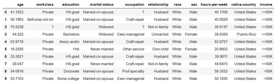 Numerical data is originally regarded as a floating point number even if it is an integer, and the data is created, so you need to convert it to an integer yourself after generation.
for col in ['age', 'hours-per-week']:
    df0_syn[col] = df0_syn[col].astype(int)
By the way, in the original paper of TGAN of the old version of CTGAN, we calculated the correlation between data items and investigated how similar the generated data is to the original data. However, let's simply compare the distribution of the target item'income' with the original data and the generated data.
print("original data")
print(df0_train['income'].value_counts(normalize=True))
# <=50K    0.759175
# >50K     0.240825

print("synthetic data")
print(df0_syn['income'].value_counts(normalize=True))
# <=50K    0.822426
# >50K     0.177574
Originally, it was non-uniform data with a small proportion of over 50K, but in the generated data, the proportion of over 50K has become even smaller. Does that mean that the distribution of the original data has not been learned so accurately? Anyway, let's check the quality of the generated data by training XGBoost.
XGBoost learning ①
Let's evaluate how similar the generated data is to the original data by training XGBoost using the generated data and comparing it with the case where the original data is used. In addition, by mixing the generated data with the original data and training it, we will try to improve the accuracy of the model compared to the case of the original data alone.
First, perform data preprocessing. This time, we will simply convert categorical variables to numbers (label encoding).
Since there may be rare variables that do not appear in a small data frame such as df_test after splitting, first use the original data frame df0 to create a dictionary containing a list of each categorical variable. Create it and apply it to each data frame using scikit-learn's LabelEncoder.
from sklearn.preprocessing import LabelEncoder
le = LabelEncoder()

category_dict = {}
for col in discrete_columns:
    category_dict[col] = df0[col].unique()

def preprocessing(df, category_dict):
    df_ = df.copy()
    for k, v in category_dict.items():
        le.fit(v)
        df_[k] = le.transform(df_[k])
    y = df_['income']
    X = df_.drop('income', axis=1)
    return X, y
Apply the function created above to each data frame.
X0_train, y0_train = preprocessing(df0_train, category_dict)
print(X0_train.shape, y0_train.shape)
# (26048, 10) (26048,)

X_test, y_test = preprocessing(df_test, category_dict)
print(X_test.shape, y_test.shape)
# (6513, 10) (6513,)

X0_syn, y0_syn = preprocessing(df0_syn, category_dict)
print(X0_syn.shape, y0_syn.shape)
# (1000000, 10) (1000000,)
We will train XGBoost and prepare a function to output the accuracy evaluation for the test data. The hyperparameters of XGBoost are determined by grid search using all data df0.
def learn_predict(X, y, X_test, y_test):
    xgb = XGBClassifier(learning_rate=0.1, max_depth=7, min_child_weight=4)
    xgb.fit(X, y)

    predictions = xgb.predict_proba(X_test)

    auc = roc_auc_score(y_test, predictions[:, 1])
    bool_pediction = (predictions[:, 1] >= 0.5).astype(int)
    acc = accuracy_score(y_test, bool_pediction)
    precision = precision_score(y_test, bool_pediction)
    recall =  recall_score(y_test, bool_pediction)
    f1 = f1_score(y_test, bool_pediction)
    print("AUC: {:.3f}".format(auc))
    print("Accuracy {:.3f}".format(acc))
    print("Precision: {:.3f}".format(precision))
    print("Recall: {:.3f}".format(recall))
    print("f1: {:.3f}".format(f1))
    print("Confusion matrix:")
    print(confusion_matrix(y_test, bool_pediction))
    return (auc, acc, precision, recall, f1)
Precision, Recall, f1 are for targets with income over 50K.
First, let's look at the results of learning with the original training data (26,048 cases). The accuracy evaluation always uses the original test data (6,513 cases) divided first.
ac0 = learn_predict(X0_train, y0_train, X_test, y_test)
# AUC: 0.888
# Accuracy:  0.838
# Precision:  0.699
# Recall  0.578
# f1:  0.632
# Confusion matrix:
# [[4554  391]
#  [ 662  906]]
We will compare this result with the result using the generated data as a baseline.
When using the generated data, learn by changing the number of samples and see how the accuracy changes depending on the number of samples.
n_samples = [1000, 3000, 10000, 30000, 100000, 300000, 1000000]
auc_list0 = []
acc_list0 = []
precision_list0 = []
recall_list0 = []
f1_list0 = []
for n in n_samples:
    print("==" * 12)
    print(" # of samples: ", n)
    print("==" * 12)
    ac = learn_predict(X0_syn[:n], y0_syn[:n], X_test, y_test)
    print()
    auc_list0.append(ac[0])
    acc_list0.append(ac[1])
    precision_list0.append(ac[2])
    recall_list0.append(ac[3])
    f1_list0.append(ac[4])
The table below shows the results.
| # of samples | 1K | 3K | 10K | 30K | 100K | 300K | 1M | Original |
|---|---|---|---|---|---|---|---|---|
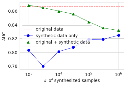
| AUC | 0.825 | 0.858 | 0.857 | 0.868 | 0.873 | 0.875 | 0.876 | 0.888 |
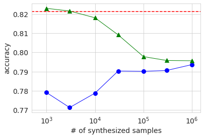
| Accuracy | 0.795 | 0.816 | 0.816 | 0.822 | 0.821 | 0.823 | 0.822 | 0.838 |
| Precision | 0.650 | 0.682 | 0.703 | 0.729 | 0.720 | 0.723 | 0.717 | 0.699 |
| Recall | 0.327 | 0.440 | 0.407 | 0.417 | 0.423 | 0.430 | 0.429 | 0.578 |
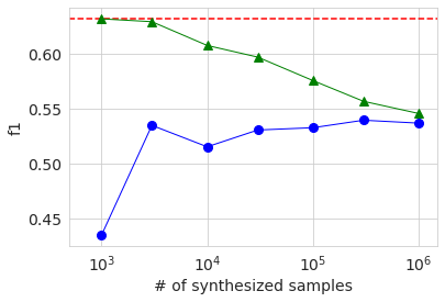
| f1 | 0.435 | 0.539 | 0.515 | 0.531 | 0.533 | 0.540 | 0.537 | 0.632 |
Although the behavior is not completely monotonous, any accuracy index tends to increase in accuracy as the number of samples increases. However, except for precision, the result of the maximum number of samples is also lower than the value of the original data. Since the accuracy evaluation is performed on the test data divided from the original data, this result suggests that the distribution of the generated data does not exactly match the original data. As far as precision is concerned, the larger the number of samples of the generated data, the better the accuracy than the original data, but this is related to the fact that the ratio of the number of samples over 50K is smaller than the original data in the generated data. I think it is.
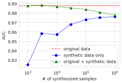
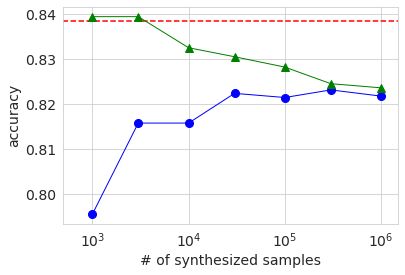
The graph below shows the results of AUC, Accuracy, and f1. The horizontal axis shows the number of samples of generated data in logarithms. The red dotted line is the result of the baseline original data, and the blue circle is the result of the generated data. The green triangle will be described later. Looking at these graphs, it can be seen that the accuracy tends to increase as the number of samples of the generated data increases, but it reaches a certain level and does not reach the result of the original data.
Next, let's train by mixing the generated data with the original data. This time as well, we are changing the number of generated data.
n_samples = [1000, 3000, 10000, 30000, 100000, 300000, 1000000]
auc_list0a = []
acc_list0a = []
precision_list0a = []
recall_list0a = []
f1_list0a = []
for n in n_samples:
    X = pd.concat([X0_train, X0_syn[:n]])
    y = pd.concat([y0_train, y0_syn[:n]])
    print("==" * 12)
    print(" # of samples: ", n)
    print("==" * 12)
    ac = learn_predict(X, y, X_test, y_test)
    print()
    auc_list0a.append(ac[0])
    acc_list0a.append(ac[1])
    precision_list0a.append(ac[2])
    recall_list0a.append(ac[3])
    f1_list0a.append(ac[4])
This result is shown in the graph above with a green triangle. When the number of samples of generated data is several thousand, which is about the same as the number of original data, the various accuracy is about the same as or slightly higher than the baseline of the original data only. However, even if it exceeds, the difference is very small, and it cannot be determined from this experiment whether it is a significant difference. If you increase the number of samples of generated data, the ratio of the original data in the data will decrease, so the accuracy will decrease, and you can see that the accuracy is asymptotic when learning only with the generated data.
XGBoost learning ②
By the way, I think that it is when the number of data that can be used for learning is small that you want to inflate data using fake data in practical situations. Assuming such a situation, let's do the same calculation using the small training data df1_train prepared first. The number of lines in df1_train is 2604, which is 1/10 of df0_train.
The code is the same as before, so I will omit it, but I trained CTGAN, generated 1 million lines of data df1_syn, and trained XGBoost.
First, the result of learning using only 2604 original baseline data is as follows.
ac1 = learn_predict(X1_train, y1_train, X_test, y_test)
# AUC: 0.867
# Accuracy:  0.821
# Precision:  0.659
# Recall  0.534
# f1:  0.590
# [[4512  433]
#  [ 730  838]]
After all, the accuracy is lowered as a whole because the number of data is reduced.
Next, the result of learning using the generated data is shown in the same graph as before.
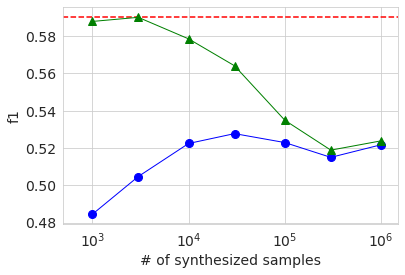
The overall behavioral trends are the same as with large datasets. The reason why the AUC and Accuracy when using only the generated data (blue circle) is lower when the number of samples is 3000 than when it is 1000 is probably because the quality of the generated data varies widely due to the small amount of original data. I guess. In any case, the accuracy was not significantly improved compared to the case of using only the original data, even if the generated data was added and learned in the same way as before.
in conclusion
I was hoping that GAN could be used to inflate the data to improve the accuracy of the model, but this experiment did not work. However, the result of using only the generated data is not so inferior to the case of using only the original data, so if the original data cannot be handled freely due to privacy or information security issues, fake data is generated instead. There may be ways to use it, such as using it for.
Recommended Posts