Google translated http://scikit-learn.org/stable/tutorial/statistical_inference/unsupervised_learning.html scikit-learn 0.18 Tutorial Table of Contents Statistical Learning Tutorial Table of Contents for Scientific Data Processing Previous tutorial page

Unsupervised learning: seeking data representation

Clustering: Group observations together

Problems solved by clustering

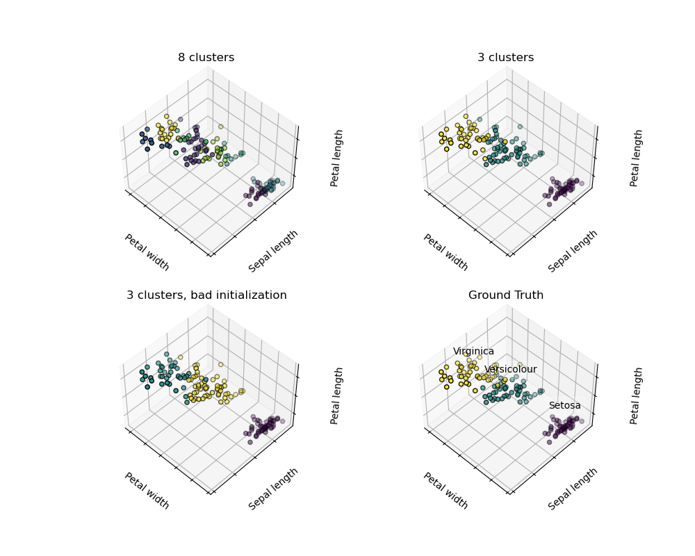
Given a iris dataset, if you have three types of iris, but you do not have access to label the taxonomists, you can try a clustering task: observes in well-separated groups called clusters. Divide.

K-means clustering

Note that there are many different clustering criteria and related algorithms. The simplest clustering algorithm is K-means (http://scikit-learn.org/stable/modules/clustering.html#k-means).

>>> from sklearn import cluster, datasets
>>> iris = datasets.load_iris()
>>> X_iris = iris.data
>>> y_iris = iris.target

>>> k_means = cluster.KMeans(n_clusters=3)
>>> k_means.fit(X_iris) 
KMeans(algorithm='auto', copy_x=True, init='k-means++', ...
>>> print(k_means.labels_[::10])
[1 1 1 1 1 0 0 0 0 0 2 2 2 2 2]
>>> print(y_iris[::10])
[0 0 0 0 0 1 1 1 1 1 2 2 2 2 2]

Warning There is absolutely no guarantee that the truth on earth will be restored. First, it's difficult to choose the right number of clusters. Second, the algorithm is sensitive to initial values, and scikit-learn uses some tricks to alleviate this problem, but it can fall within the local minimum.

Bad initialization	8 clusters	Ground truth

** Do not over-interpret clustering results **

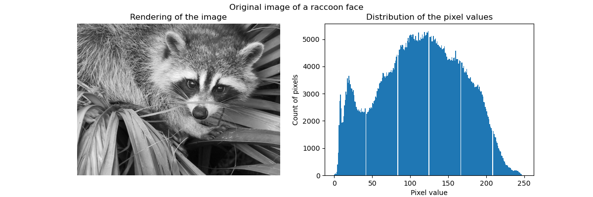
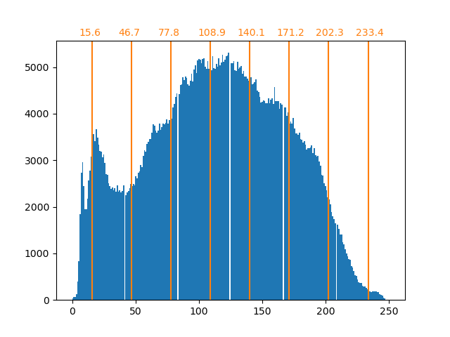
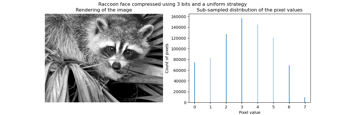
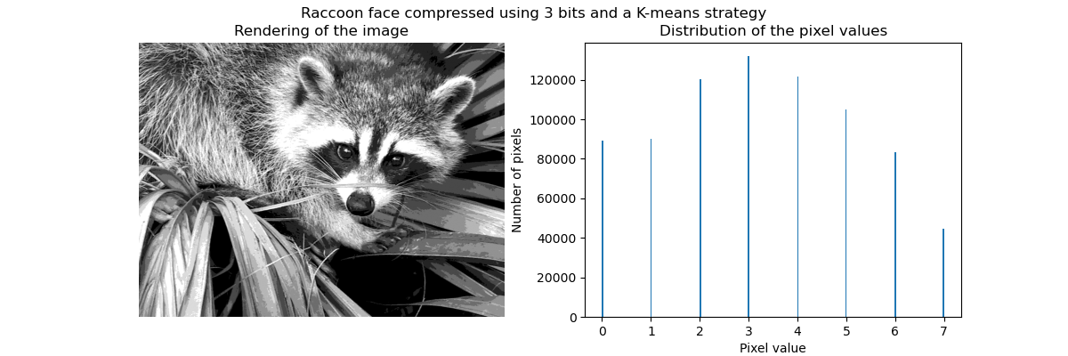
Application example: Vector quantization

In general, clustering and KMeans can be seen as a way to choose a few examples for compressing information. This problem is sometimes referred to as vector quantization. For example, this can be used to posterize an image:

>>> import scipy as sp
>>> try:
...    face = sp.face(gray=True)
... except AttributeError:
...    from scipy import misc
...    face = misc.face(gray=True)
>>> X = face.reshape((-1, 1)) # We need an (n_sample, n_feature) array
>>> k_means = cluster.KMeans(n_clusters=5, n_init=1)
>>> k_means.fit(X) 
KMeans(algorithm='auto', copy_x=True, init='k-means++', ...
>>> values = k_means.cluster_centers_.squeeze()
>>> labels = k_means.labels_
>>> face_compressed = np.choose(labels, values)
>>> face_compressed.shape = face.shape

Raw image	K-Quantization	Equal bin	Image histogram

Hierarchical cohesive clustering: Ward's method

Hierarchical clustering is a type of cluster analysis that aims to build a hierarchy of clusters. In general, the various approaches of this technique

-** Aggregate -Bottom-up approach: Each observation starts with its own cluster, and the clusters are intensively merged in such a way as to minimize the binding criteria. This approach is especially interesting when the clusters of interest are made up of very few observations. With a large number of clusters, it is much more computationally efficient than the k-means. -- Branched ** --Top-down approach: All observations start in one cluster and are iteratively divided as you move through the hierarchy. To estimate a large number of clusters, this approach is slow and statistically malicious (for all observations starting as one cluster and splitting recursively).

Clustering with constrained connectivity

Aggregate clustering allows you to specify which samples to cluster by creating a connection graph. The graph in scikit is represented by its adjacency matrix. Sparse matrices are often used. This is useful, for example, when clustering images to get the connected area (also known as the connected component).

import matplotlib.pyplot as plt

from sklearn.feature_extraction.image import grid_to_graph
from sklearn.cluster import AgglomerativeClustering
from sklearn.utils.testing import SkipTest
from sklearn.utils.fixes import sp_version

if sp_version < (0, 12):
    raise SkipTest("Skipping because SciPy version earlier than 0.12.0 and "
                   "thus does not include the scipy.misc.face() image.")


###############################################################################
# Generate data
try:
    face = sp.face(gray=True)
except AttributeError:
    # Newer versions of scipy have face in misc
    from scipy import misc
    face = misc.face(gray=True)

# Resize it to 10% of the original size to speed up the processing
face = sp.misc.imresize(face, 0.10) / 255.

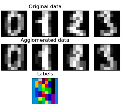
Aggregation of features

We have found that the curse of dimensional numbers, i.e., can be used to alleviate inadequate observations compared to the number of features. Another approach is to integrate similar features. Agglomeration of features. This approach can be achieved by feature-oriented clustering, in other words clustering of transposed data.

>>> digits = datasets.load_digits()
>>> images = digits.images
>>> X = np.reshape(images, (len(images), -1))
>>> connectivity = grid_to_graph(*images[0].shape)

>>> agglo = cluster.FeatureAgglomeration(connectivity=connectivity,
...                                      n_clusters=32)
>>> agglo.fit(X) 
FeatureAgglomeration(affinity='euclidean', compute_full_tree='auto',...
>>> X_reduced = agglo.transform(X)

>>> X_approx = agglo.inverse_transform(X_reduced)
>>> images_approx = np.reshape(X_approx, images.shape)

`transform` method and ʻinverse_transform` method

Some estimators expose the transform method, for example, to reduce the number of dimensions in a dataset.

Decomposition: from signal to component and loading

Components and loading

If X is our multivariate data, the problem we are trying to solve is to rewrite it with different observation criteria: we like loading $ L $ and $ X = LC $. I want to learn a set of components $ C $. There are different criteria for selecting components.

Principal component analysis: PCA

Principal Component Analysis (PCA) (http://scikit-learn.org/stable/modules/decomposition.html#pca) selects continuous components that describe the maximum variance of the signal.

The point cloud that spans the above observations is very flat in one direction. One of the three univariate features can be calculated almost exactly using the other two functions. PCA finds directions where data is not flat PCA can be used to transform data to reduce the dimensions of the data by projecting it into a major subspace.

>>> #Create a signal with only two valid dimensions
>>> x1 = np.random.normal(size=100)
>>> x2 = np.random.normal(size=100)
>>> x3 = x1 + x2
>>> X = np.c_[x1, x2, x3]

>>> from sklearn import decomposition
>>> pca = decomposition.PCA()
>>> pca.fit(X)
PCA(copy=True, iterated_power='auto', n_components=None, random_state=None,
  svd_solver='auto', tol=0.0, whiten=False)
>>> print(pca.explained_variance_)  
[  2.18565811e+00   1.19346747e+00   8.43026679e-32]

>>> #As you can see, only the first two components are useful
>>> pca.n_components = 2
>>> X_reduced = pca.fit_transform(X)
>>> X_reduced.shape
(100, 2)

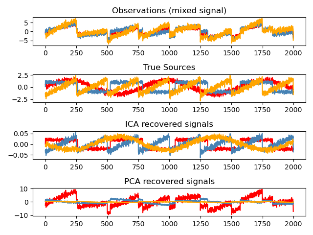
Independent component analysis: ICA

Independent Component Analysis (ICA) (http://scikit-learn.org/stable/modules/decomposition.html#ica) selects components so that the distribution of the components carries the maximum amount of independent information. .. ** Non-Gauss ** Independent signals can be restored.

>>> # Generate sample data
>>> time = np.linspace(0, 10, 2000)
>>> s1 = np.sin(2 * time)  # Signal 1 : sinusoidal signal
>>> s2 = np.sign(np.sin(3 * time))  # Signal 2 : square signal
>>> S = np.c_[s1, s2]
>>> S += 0.2 * np.random.normal(size=S.shape)  # Add noise
>>> S /= S.std(axis=0)  # Standardize data
>>> # Mix data
>>> A = np.array([[1, 1], [0.5, 2]])  # Mixing matrix
>>> X = np.dot(S, A.T)  # Generate observations

>>> # Compute ICA
>>> ica = decomposition.FastICA()
>>> S_ = ica.fit_transform(X)  # Get the estimated sources
>>> A_ = ica.mixing_.T
>>> np.allclose(X,  np.dot(S_, A_) + ica.mean_)
True

[PYTHON] [Translation] scikit-learn 0.18 Tutorial Statistical learning tutorial for scientific data processing Unsupervised learning: Finding the representation of data