[PYTHON] [Translation] scikit-learn 0.18 tutorial Statistical learning tutorial for scientific data processing Supervised learning: Predicting output variables from high-dimensional observations
Google Translated http://scikit-learn.org/0.18/tutorial/statistical_inference/supervised_learning.html scikit-learn 0.18 Tutorial Table of Contents Statistical Learning Tutorial Table of Contents for Scientific Data Processing Previous page
Supervised learning: predicting output variables from high-dimensional observations
Problems solved by supervised learning
[Supervised learning](http://qiita.com/nazoking@github/items/267f2371757516f8c168#1-%E6%95%99%E5%B8%AB%E4%BB%98%E3%81%8D%E5 % AD% A6% E7% BF% 92) is the link between the observation data X and the external variable y (usually called the "target" or "label") that you are trying to predict. Is to learn. Often, y is a one-dimensional array of length n_samples.
All scikit-learn supervised estimators have a fit (X, y) method that fits the model and a predict (returns the predictive label ygiven the unlabeled observationX. Implement the X) method.
Vocabulary: Classification and Regression
If the predictive task is to classify observations within a series of finite labels, in other words the task of "naming" the observed objects is called a ** classification ** task. On the other hand, if the goal is to predict a continuous goal variable, it is said to be a ** regression ** task.
When classifying with scikit-learn, y is a vector of integers or strings.
Note: For an easy way to implement the basic machine learning vocabulary used in scikit-learn, see Introduction to Machine Learning with the scikit-learn tutorial. ae16bd4d93464fbfa19b) ".
Nearest neighbor and curse of dimensionality
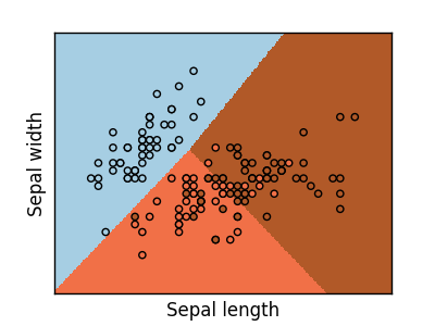
Categorize iris:
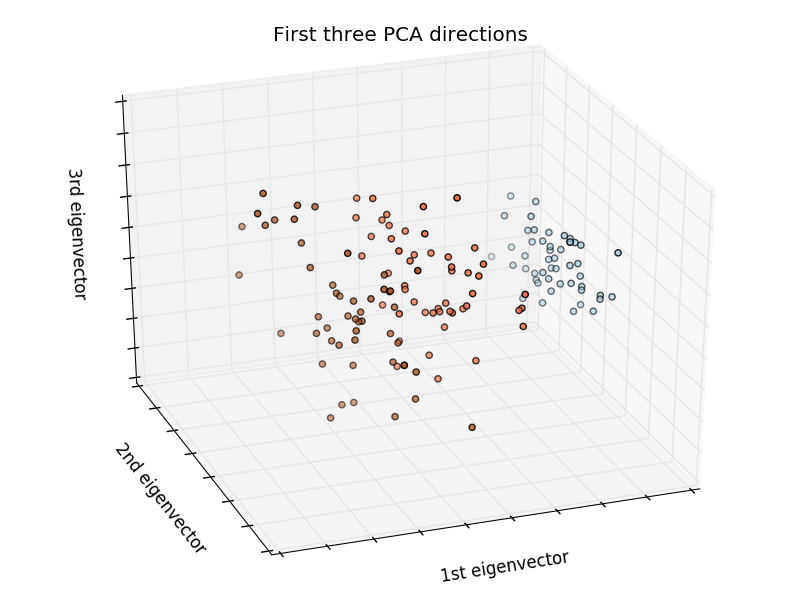
The iris dataset is a classification task that identifies iris types (Setosa, Versicolour, and Virginia) by petal and leaf length and width.
>>> import numpy as np
>>> from sklearn import datasets
>>> iris = datasets.load_iris()
>>> iris_X = iris.data
>>> iris_y = iris.target
>>> np.unique(iris_y)
array([0, 1, 2])
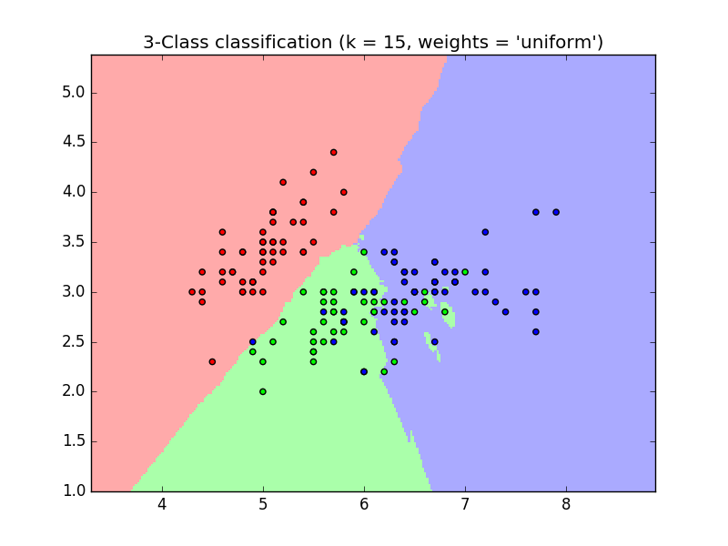
k-nearest neighbor classifier
The simplest possible classifier is the Nearest Neighbor (https://en.wikipedia.org/wiki/K-nearest_neighbor_algorithm). Given a new sample X_test, find observations with the closest feature vector in the training set (ie, the data used to train the estimator). (For more information on this type of classifier, see the "Nearest Neighbors" section of the Scikit-online online manual. Please give me).
Training set and test set
While experimenting with any training algorithm, it is important not to test the data used for training so that you can evaluate the estimator performance on the new data. For this reason, datasets are often split into training and test data.
KNN (k-nearest neighbor) classification example:
>>> #Split iris data into training data and test data
>>> #Random permutation that randomly divides the data
>>> np.random.seed(0)
>>> indices = np.random.permutation(len(iris_X))
>>> iris_X_train = iris_X[indices[:-10]]
>>> iris_y_train = iris_y[indices[:-10]]
>>> iris_X_test  = iris_X[indices[-10:]]
>>> iris_y_test  = iris_y[indices[-10:]]
>>> #Create and fit the nearest neighbor classifier
>>> from sklearn.neighbors import KNeighborsClassifier
>>> knn = KNeighborsClassifier()
>>> knn.fit(iris_X_train, iris_y_train)
KNeighborsClassifier(algorithm='auto', leaf_size=30, metric='minkowski',
           metric_params=None, n_jobs=1, n_neighbors=5, p=2,
           weights='uniform')
>>> knn.predict(iris_X_test)
array([1, 2, 1, 0, 0, 0, 2, 1, 2, 0])
>>> iris_y_test
array([1, 1, 1, 0, 0, 0, 2, 1, 2, 0])
Curse of dimensionality
For the estimator to be effective, the distance between adjacent points must be less than a certain value, $ d $, depending on the problem. In one dimension, this requires an average of $ n ~ 1 / d $ points. In the $ k $ -nearest neighbor example above, the data is described by only one feature with a value in the range 0 to 1, and in $ n $ training observations, the new data is no more than $ 1 / n $. .. Therefore, if $ 1 / n $ is small compared to the magnitude of the variation of interclass features, the nearest neighbor determination rule is efficient. If the number of features is $ p $, you need $ n to 1 / d ^ p $ points. Let's say you need 10 points in one dimension. Here we need $ 10 ^ p $ points in the $ p $ dimension to pave the $ [0, 1] $ space. As $ p $ grows, the number of training points required for a good estimator increases exponentially. For example, if each point is just a number (8 bytes), a valid $ k $ -nearest neighbor estimator requires more training data than the current estimated size of the entire Internet (± 1000 Exabytes or more). .. This is called the Curse of Dimensionality (https://en.wikipedia.org/wiki/Curse_of_dimensionality) and is a central issue that machine learning addresses.
Linear model: from regression to sparseness
Diabetes dataset
The diabetes dataset consists of 10 physiological variables (age, gender, weight, blood pressure) in 442 patients, and indicators of disease progression after 1 year:
>>> diabetes = datasets.load_diabetes()
>>> diabetes_X_train = diabetes.data[:-20]
>>> diabetes_X_test  = diabetes.data[-20:]
>>> diabetes_y_train = diabetes.target[:-20]
>>> diabetes_y_test  = diabetes.target[-20:]
The current challenge is to predict disease progression from physiological variables.
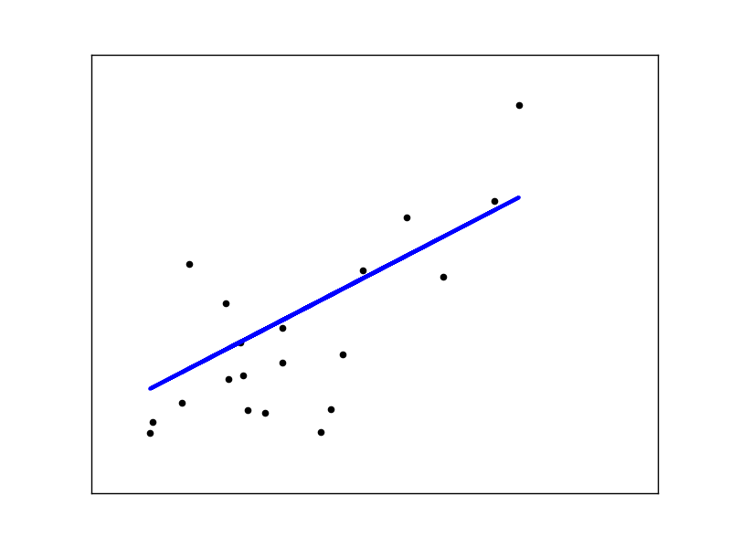
Linear regression
LinearRegression is the simplest form of sum of squares of model residuals. Fit the linear model to the dataset by adjusting a set of parameters to make it as small as possible.
Linear model: $ y = X \ beta + ε $
-$ X
>>> from sklearn import linear_model
>>> regr = linear_model.LinearRegression()
>>> regr.fit(diabetes_X_train, diabetes_y_train)
LinearRegression(copy_X=True, fit_intercept=True, n_jobs=1, normalize=False)
>>> print(regr.coef_)
[   0.30349955 -237.63931533  510.53060544  327.73698041 -814.13170937
  492.81458798  102.84845219  184.60648906  743.51961675   76.09517222]

>>> #Mean squared error
>>> np.mean((regr.predict(diabetes_X_test)-diabetes_y_test)**2)
2004.56760268...

>>> #Explained variance score: 1 is a perfect prediction and 0 means there is no linear relationship between X and y.
>>> regr.score(diabetes_X_test, diabetes_y_test)
0.5850753022690...
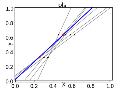
Shrink
If there are few data points per dimension, the noise in the observations causes a high variance.
X = np.c_[ .5, 1].T
y = [.5, 1]
test = np.c_[ 0, 2].T
regr = linear_model.LinearRegression()

import matplotlib.pyplot as plt
plt.figure()

np.random.seed(0)
for _ in range(6):
   this_X = .1*np.random.normal(size=(2, 1)) + X
   regr.fit(this_X, y)
   plt.plot(test, regr.predict(test))
   plt.scatter(this_X, y, s=3)
The solution for higher-order statistical learning is to reduce the regression coefficients to zero. Any two randomly selected observation sets can be uncorrelated. This is called ridge regression.
>>> regr = linear_model.Ridge(alpha=.1)

>>> plt.figure()

>>> np.random.seed(0)
>>> for _ in range(6):
...    this_X = .1*np.random.normal(size=(2, 1)) + X
...    regr.fit(this_X, y)
...    plt.plot(test, regr.predict(test))
...    plt.scatter(this_X, y, s=3)
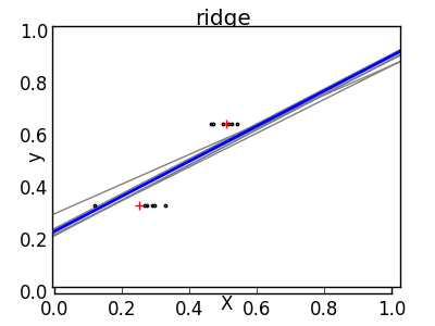
This is an example of a bias / dispersion trade-off. The larger the ridge ʻalpha parameter, the higher the bias and the smaller the variance. You can select ʻalpha to minimize miss-out errors. This time, we are using the diabetes dataset instead of the synthetic data.
>>> alphas = np.logspace(-4, -1, 6)
>>> from __future__ import print_function
>>> print([regr.set_params(alpha=alpha
...             ).fit(diabetes_X_train, diabetes_y_train,
...             ).score(diabetes_X_test, diabetes_y_test) for alpha in alphas])
[0.5851110683883..., 0.5852073015444..., 0.5854677540698..., 0.5855512036503..., 0.5830717085554..., 0.57058999437...]
** Note: ** Capturing noise that prevents the model from being generalized to new data with matched parameters is called Overfitting (https://en.wikipedia.org/wiki/Overfitting). The bias introduced by Ridge Regression is called Regularization (https://en.wikipedia.org/wiki/Regularization_%28machine_learning%29).
Diluteness
Fitting Feature 1 and Feature 2 only
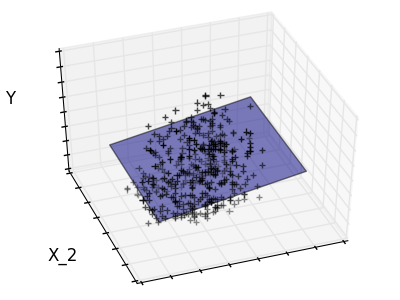
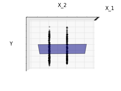
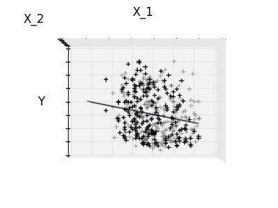
Feature 2 has a strong coefficient for the full model, but when considered for feature 1, it can be seen that it conveys very little information about y. It would be interesting to select only useful features and set 0 for non-beneficial features such as feature 2 to improve the situation in question (ie, mitigate the curse of dimensionality). Ridge regression reduces their contributions, but does not set them to zero. Another penalty approach, called the Lasso (Minimum Absolute Reduction and Selection Operator), allows you to set some coefficients to zero. Such a method is called the sparse method, and the dilution can be seen as an application of Occam's razor.
>>> regr = linear_model.Lasso()
>>> scores = [regr.set_params(alpha=alpha
...             ).fit(diabetes_X_train, diabetes_y_train
...             ).score(diabetes_X_test, diabetes_y_test)
...        for alpha in alphas]
>>> best_alpha = alphas[scores.index(max(scores))]
>>> regr.alpha = best_alpha
>>> regr.fit(diabetes_X_train, diabetes_y_train)
Lasso(alpha=0.025118864315095794, copy_X=True, fit_intercept=True,
   max_iter=1000, normalize=False, positive=False, precompute=False,
   random_state=None, selection='cyclic', tol=0.0001, warm_start=False)
>>> print(regr.coef_)
[   0.         -212.43764548  517.19478111  313.77959962 -160.8303982    -0.
 -187.19554705   69.38229038  508.66011217   71.84239008]
Different algorithms for the same problem
Different algorithms can be used to solve the same mathematical problem. For example, the scikit-learn Lasso object solves the Lasso regression problem using the efficient Coordinate Descent method (https://en.wikipedia.org/wiki/Coordinate_descent) on large datasets. I will. However, scikit-learn uses LARS algorthm to provide the LassoLars object. To do. This is very efficient for problems with very sparse estimated weight vectors (problems with very few observations).
Classification
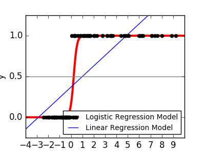
As with the iris classification task, linear regression is not a good approach as it puts a great deal of weight on data far from the decision frontier. The linear approach is to fit sigmoid or logistic functions.
y = \textrm{sigmoid}(X\beta - \textrm{offset}) + \epsilon =
\frac{1}{1 + \textrm{exp}(- X\beta + \textrm{offset})} + \epsilon
>>> logistic = linear_model.LogisticRegression(C=1e5)
>>> logistic.fit(iris_X_train, iris_y_train)
LogisticRegression(C=100000.0, class_weight=None, dual=False,
          fit_intercept=True, intercept_scaling=1, max_iter=100,
          multi_class='ovr', n_jobs=1, penalty='l2', random_state=None,
          solver='liblinear', tol=0.0001, verbose=0, warm_start=False)
This is called LogisticRegression.
Multi-class classification
If you have multiple classes to predict, a common option is to fit one-to-all classifiers before using voting heuristics for the final decision.
Shrinkage and thinness due to logistic regression
The C parameter controls the amount of normalization of the LogisticRegression object. Larger C values result in less regularization. penalty =" l2 " gives contraction (ie, non-sparse coefficient) and penalty =" l2 " gives sparseness.
Exercise
Try classifying the numeric dataset using the nearest neighbor and linear models. Test these observations, leaving the last 10%.
from sklearn import datasets, neighbors, linear_model

digits = datasets.load_digits()
X_digits = digits.data
y_digits = digits.target
Support Vector Machine (SVM)
Linear SVM
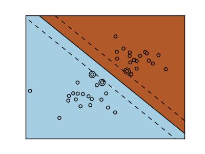
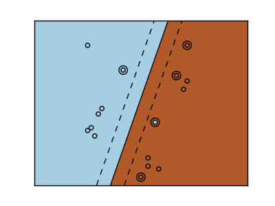
The support vector machine belongs to the discriminant model group. Find a combination of samples and try to build a plane that maximizes the margin between the two classes. Regularization is set by the C parameter. A small value for C means that the margin is calculated using many or all of the observations around the dividing line (further regularization). If the value of C is large, it means that the margin is calculated (less regularization) with the observed value close to the dividing line.
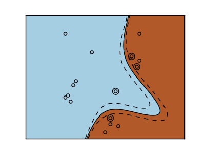
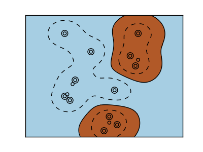
| Regularized SVM | Regularized SVM(Default) |
|---|---|
 |
 |
--Example: -Plot different SVM classifiers on iris dataset
SVM Regression-SVR (Support Vector Regression)-or Classification-[SVC] It can be used at (http://scikit-learn.org/0.18/modules/generated/sklearn.svm.SVC.html#sklearn.svm.SVC) (Support Vector Classification).
>>> from sklearn import svm
>>> svc = svm.SVC(kernel='linear')
>>> svc.fit(iris_X_train, iris_y_train)
SVC(C=1.0, cache_size=200, class_weight=None, coef0=0.0,
    decision_function_shape=None, degree=3, gamma='auto', kernel='linear',
    max_iter=-1, probability=False, random_state=None, shrinking=True,
    tol=0.001, verbose=False)
Using the kernel
Classes cannot always be linearly separated in the feature space. The solution is to build a decision function that is a polynomial rather than a linear one. This is done using a kernel trick that can be considered to generate decision energy by placing the kernel in the observation.
Linear kernel
>>> svc = svm.SVC(kernel='linear')
Polynomial kernel
>>> svc = svm.SVC(kernel='poly',
...               degree=3)
>>> # degree:Polynomial degree
RBF kernel (Radial Basis Function)
>>> svc = svm.SVC(kernel='rbf')
>>> # gamma:Reciprocal of radial kernel size
Interactive example
To download svm_gui.py, SVM GUI Please refer to. Add data points for both classes with the right and left buttons to fit the model and change the parameters and data.
Exercise
Try classifying Class 1 and Class 2 from the Iris dataset with an SVM that has two first features. Based on these observations, we test predictive performance, leaving 10% of each class.
WARNING: Classes are ordered and do not leave the last 10%. You only test in one class. Tip: You can get intuition by using the decision_function method on the grid.
iris = datasets.load_iris()
X = iris.data
y = iris.target

X = X[y != 0, :2]
y = y[y != 0]
Next page © 2010 --2016, scikit-learn developers (BSD license).
Recommended Posts