[PYTHON] [Translation] NumPy Official Tutorial "NumPy: the absolute basics for beginners"

Introduced by the translator

This article is a translation of "NumPy: the absolute basics for beginners" in the official NumPy v.1.19 Documentation. This document was released after the development version was changed to this release.

Python has remained very popular in recent years. One of the reasons is the AI boom and the richness of Python's machine learning libraries. It seems that Python's abundant libraries in the field of scientific and technological calculations such as machine learning are causing further expansion of the library and support not limited to beginners.

NumPy is the underlying system for these scientific and technological computational libraries. The reason why NumPy is adopted is the speed issue of Python. Due to the nature of the language, Python is known to be very slow for some operations. Therefore, many libraries use NumPy implemented in C language to avoid the processing bottleneck of Python speed, and realize the speed that can withstand a large amount of data processing. is.

NumPy has the appeal of being very convenient and fast, but it can be a bit tricky compared to Python itself. In this article, I explain the basics of NumPy clearly with images. The scope of the explanation covers more than half of "Quickstart tutorial", so read that dry tutorial. You should be able to do some things at least.

You may also find it helpful to read [For beginners] Illustrated NumPy and data representation. The author is the creator of the images in this article. It would be greatly appreciated if you could point out any mistranslations.

** Translated below **

Welcome to the guide to NumPy complete beginners! If you have any comments or suggestions, feel free to contact us!

Welcome to NumPy!

NumPy (Numerical Python) is an open source Python library used in almost every area of science and engineering. Numpy is the global standard for working with numerical data and is the core of Scientific Python and the Pydata family [Pydata ecosystems: Numpy developer Pydata's product line]. NUmpy users range from novice programmers to veteran researchers doing cutting-edge scientific and engineering research and development. The Numpy API is widely used in Pandas, SciPy, Matplotlib, scikit-learn, scikit-image and most other data science and scientific Python packages. The Numpy library has multidimensional array and matrix data structures (more on this in a later section). Numpy provides ndarray, an n-dimensional array object of the same type [same data type], along with methods for processing arrays efficiently. Numpy can be used to perform a variety of mathematical operations on arrays. Numpy adds powerful data structures to Python that guarantee efficient computation of arrays and matrices, and provides a huge library with advanced mathematical capabilities that work with these arrays and matrices. Learn more about NumPy here!

Install NumPy

We strongly recommend using a scientific Python distribution to install NumPy. if If you need complete guidance on installing NumPy on your OS, here you can find all the details (https://www.scipy.org/install.html).

If you are already using Python, you can install NumPy with the following code.

conda install numpy

Or

pip install numpy

If you don't have Python yet, you should consider using Anaconda. Anaconda is the easiest way to get started with Python. The advantage of using this distribution is that you don't have to worry too much about installing NumPy, the main packages used for data analysis, pandas, Scikit-Learn, etc. individually.

You can find all of the installation details in the InstallationsectionatSciPy.

How to import NumPy

Whenever you want to use a package or library, you need to make the first one accessible. To get started with NumPy and all its features, you have to import NumPy. This can be easily done with the following import statement [statement].

import numpy as np

(We abbreviate NumPy as np, to save time, and to standardize the code so that anyone working with it can easily understand and execute it. .)

How to read the code example

If your code isn't used to reading a lot of tutorials, you may not know how to understand a code block like this:

>>> a = np.arange(6)
>>> a2 = a[np.newaxis, :]
>>> a2.shape
(1, 6)

Even if you are not familiar with this method, this notation is very easy to understand. If there is >>>, it points to ** input **, that is, the code you will enter. Anything without >>> in front of the code is ** output **, the result of executing the code. This is the style when running Python on the command line, but when using IPython you may see different styles.

What's the difference between a Python list and a NumPy array?

NumPy has numerous fast and efficient ways to create arrays and manipulate numeric data. Pyhon lists can have different data types in one list, but in a NumPy array all the elements on the array must be of the same type. If the array is mixed with other data types, the mathematical operations that should work on the array will be severely inefficient.

Why is NumPy used?

NumPy arrays are faster and more concise than Python lists. [Python] arrays use less memory and are convenient to use. By comparison, NumPy uses much less memory to store data and has a mechanism for identifying data types. This allows for further optimization of the code.

What is an array?

Arrays are one of the main data structures in the NumPy library. An array is a grid of values, and an array has information about the raw data, information about how to arrange the elements, and information about how to interpret the elements. A grid of elements that NumPy has can be indexed in various ways. I will. The elements are all homogeneous and are represented as dtype in the array.

Arrays can be indexed by a tuple of positive integers, booleans, another array or an integer. The rank of the array is the number of dimensions. The shape of an array is an integer tuple that represents the size of the array along each dimension. One way to initialize a NumPy array is to initialize it from a Python list. Use a nested list for data in two or more dimensions.

Example:

>>> a = np.array([1, 2, 3, 4, 5, 6])

Or

>>> a = np.array([[1, 2, 3, 4], [5, 6, 7, 8], [9, 10, 11, 12]])

Use brackets to access the elements of the array. Remember that NumPy indexes start at 0 when accessing the elements of an array. This means that if you want to access the first element of the array, you will be accessing the array "0".

>>> print(a[0])
[1 2 3 4]

Learn more about arrays

• This section deals with 1D array, 2D array, ndarray, vector, matrix *

You may have occasionally seen an array labeled "ndarray". This is an abbreviation for "N-dimensional array". An N-dimensional array is simply an array with an arbitrary number of dimensions. You may also have seen "** 1-D " or one-dimensional arrays, " 2-D **" or two-dimensional arrays, etc ... NumPy's ndarray class is used to represent both matrices and vectors. ** Vector ** is a one-dimensional array (there is no difference between row and column vectors), and ** matrix ** refers to a two-dimensional array. The term ** tensor ** is also often used for arrays of ** 3D ** and above.

** What are array attributes? ** **

Arrays are usually fixed-size containers of items of the same type and size. The number of dimensions and items of an array are defined by the shape of the array. The shape of the array is a tuple of natural numbers that defines the size of each dimension. In NumPy, dimensions are called ** axes **. That is, if you have the following array

[[0., 0., 0.],
 [1., 1., 1.]]

This array has two axes. The length of the first axis is 2 and the length of the second is 3. As with any Python container, you can access and modify the contents of the array with indexes and slicing. But unlike typical container objects, the same data can be shared in different arrays, so changes made in one array may appear in another.

The ** attributes ** of an array reflect array-specific information. If you need to get or set array properties without creating a new array, you often access the array through the attributes of the array.

Read more about array attributes hereandlearnaboutarrayobjectshere.

How to make a simple array

_ In this section np.array (), np.zeros (), np.ones (), np.empty (), np.arange (), np.linspace () , dtype is handled_

To create a NumPy array, use the function np.array (). All you need to do to make a simple array is pass a list. You can also specify the list data type if desired. You can find more information about data types here.

>>> import numpy as np
>>> a = np.array([1, 2, 3])

You can visualize the array as follows: Keep in mind that these visualizations are meant to make the concept easier to understand and give you a basic understanding of how NumPy comes up and works. Arrays and array operations are much more complex than those represented here. In addition to the array created from a series of elements, you can easily create an array filled with 0.

>>> np.zeros(2)
array([0., 0.])

You can also create an array filled with 1.

>>> np.ones(2)
array([1., 1.])

Or even an empty array! The ʻempty function creates an array whose initial contents are random and depend on the state of memory. The reason for using the ʻempty function over the zero function (or something similar) is speed. Don't forget to fill in all the elements later!

>>> # Create an empty array with 2 elements
>>> np.empty(2)
array([ 3.14, 42.  ])  # may vary

You can create an array of contiguous elements:

>>> np.arange(4)
array([0, 1, 2, 3])

You can also create an array of evenly spaced columns. To do so, specify ** first number **, ** last number **, and number of steps.

>>> np.arange(2, 9, 2)
array([2, 4, 6, 8])

You can use np.linspace () to create an array with linearly spaced values at specified intervals.

>>> np.linspace(0, 10, num=5)
array([ 0. ,  2.5,  5. ,  7.5, 10. ])

** Specify the data type **

The default data type is floating point (np.float64), but you can explicitly specify the data type you want to use with the dtype keyword.

>>> x = np.ones(2, dtype=np.int64)
>>> x
array([1, 1])

Learn more about creating arrays here

Add / remove / sort elements

• This section deals with np.sort (), np.concatenate () *

When sorting elements, it's easy to use np.sort (). When calling this function, you can specify the axis, type, and order.

Taking this array as an example,

>>> arr = np.array([2, 1, 5, 3, 7, 4, 6, 8])

In this way, you can quickly sort in ascending order.

>>> np.sort(arr)
array([1, 2, 3, 4, 5, 6, 7, 8])

sort returns a sorted copy into an array, but you can also use: · ʻArgsort](https://numpy.org/doc/stable/reference/generated/numpy.argsort.html#numpy.argsort): Indirect sorting by the specified axis · [Lexsort](https://numpy.org/doc/stable/reference/generated/numpy.lexsort.html#numpy.lexsort): Indirect stable sort on multiple keys] · [Searchsorted](https://numpy.org/doc/stable/reference/generated/numpy.searchsorted.html#numpy.searchsorted): Discover elements from a sorted array -[Partition`: Partial sort

Take these arrays as an example:

>>> a = np.array([1, 2, 3, 4])
>>> b = np.array([5, 6, 7, 8])

You can concatenate these arrays with np.concatenate ().

>>> np.concatenate((a, b))
array([1, 2, 3, 4, 5, 6, 7, 8])

Also, taking this array as an example:

>>> x = np.array([[1, 2], [3, 4]])
>>> y = np.array([[5, 6]])

This way you can concatenate:

>>> np.concatenate((x, y), axis=0)
array([[1, 2],
       [3, 4],
       [5, 6]])

To remove an element from the array, it's easy to use the index to select the element you want to keep. If you want to know more about concatenation, see right: concatenate.

How to know the shape and size of an array?

• This section deals with ndarray.ndim, ndarray.size, ndarray.shape *

ndarray.ndim indicates the number of axes in the array, that is, the number of dimensions.

ndarray.size shows the total number of elements in the array. This is the product of the size of the array.

ndarray.shape displays an integer tuple that indicates the number of elements stored in each dimension of the array. For example, if you have a 2D, 3D array, the shape of the array is (2,3).

For example, suppose you create the following array:

>>> array_example = np.array([[[0, 1, 2, 3],
...                           [4, 5, 6, 7]],
...                          [[0, 1, 2, 3],
...                           [4, 5, 6, 7]],
...                          [[0 ,1 ,2, 3],
...                           [4, 5, 6, 7]]])

To find out the number of dimensions in an array, do the following:

>>> array_example.ndim
3

To find out the total number of elements in an array, do the following:

>>> array_example.size
24

And to find out the shape of the array, do the following:

>>> array_example.shape
(3, 2, 4)

Can I transform the array?

• This section deals with ʻarr.reshape () `*

of course! You can use ʻarr.reshape () `to give an array a new shape without changing the data. When using this transformation method, keep in mind that the array you want to create must have the same number of elements as the original array. If you transform an array of 12 elements, you need to make sure that the new array also has a total of 12 elements. If you use this array:

>>> a = np.arange(6)
>>> print(a)
[0 1 2 3 4 5]

You can use reshape () to transform the array. For example, you can transform this array into a 3-by-2 array:

>>> b = a.reshape(3, 2)
>>> print(b)
[[0 1]
 [2 3]
 [4 5]]

It is possible to specify some parameters with np.shape (). ::

>>> numpy.reshape(a, newshape=(1, 6), order='C')]
array([[0, 1, 2, 3, 4, 5]])

ʻAis an array that changes shape. newshape is the shape of the new array. You can specify an integer or an integer tuple. If you specify an integer, an array of that integer length is created. The shape must be compatible with the original shape. ʻOrder: C stands for reading and writing in a C-like index order, and F means reading and writing in a Fortran-like index order. A means use a Fortran-like index order if the element is Fortran contiguous in memory, otherwise use a C-like index (this is an optional parameter and must be specified. No need to). If you want to learn more about C and Fortran order, you can read more about the internal organization of NumPy arrays here. Essentially, C and Fortran orders have to do with how indices correspond to the order the array is stored in memory. In Fortran, when moving through the elements of a two-dimensional array as it is stored in memory, the first index is the most rapidly varying index. As the first index moves to the next row as it changes, the matrix is stored one column at a time. This is why Fortran is thought of as a Column-major language. In C on the other hand, the last index changes the most rapidly. The matrix is stored by rows, making it a Row-major language. What you do for C or Fortran depends on whether it’s more important to preserve the indexing convention or not reorder the data. Learn more about shape manipulation here.

How to convert a 1D array to a 2D array (how to add a new axis to an array)

• This section deals with np.newaxis, np.expand_dims *

You can use np.newaxis and np.expand_dims to increase the dimensions of an existing array.

Using np.newaxis increases the dimension of the array by one dimension when used only once. That is, a 1D array becomes a 2D array, a 2D array becomes a 3D array, and so on.

For example, in the following array

>>> a = np.array([1, 2, 3, 4, 5, 6])
>>> a.shape
(6,)

You can add a new axis using np.newaxis. ::

>>> a2 = a[np.newaxis, :]
>>> a2.shape
(1, 6)

You can explicitly transform a 1D array from either a row vector or a column vector by using np.newaxis. For example, you can convert a 1D array to a row vector by inserting an axis in the first dimension.

>>> row_vector = a[np.newaxis, :]
>>> row_vector.shape
(1, 6)

You can also insert axes in the second dimension into column vectors:

>>> col_vector = a[:, np.newaxis]
>>> col_vector.shape
(6, 1)

You can also expand the array by inserting the axes specified in np.expand_dims. For example, in this array:

>>> a = np.array([1, 2, 3, 4, 5, 6])
>>> a.shape
(6,)

You can use np.expand_dims to add an axis at index position 1. ::

>>> b = np.expand_dims(a, axis=1)
>>> b.shape
(6, 1)

To add an axis at index position 0: ::

>>> c = np.expand_dims(a, axis=0)
>>> c.shape
(1, 6)

Indexing and slicing

Subscript access and slicing of Numpy arrays can be done in the same way as slicing Python lists.

>>> data = np.array([1, 2, 3])

>>> data[1]
2
>>> data[0:2]
array([1, 2])
>>> data[1:]
array([2, 3])
>>> data[-2:]
array([2, 3])

This can be visualized as: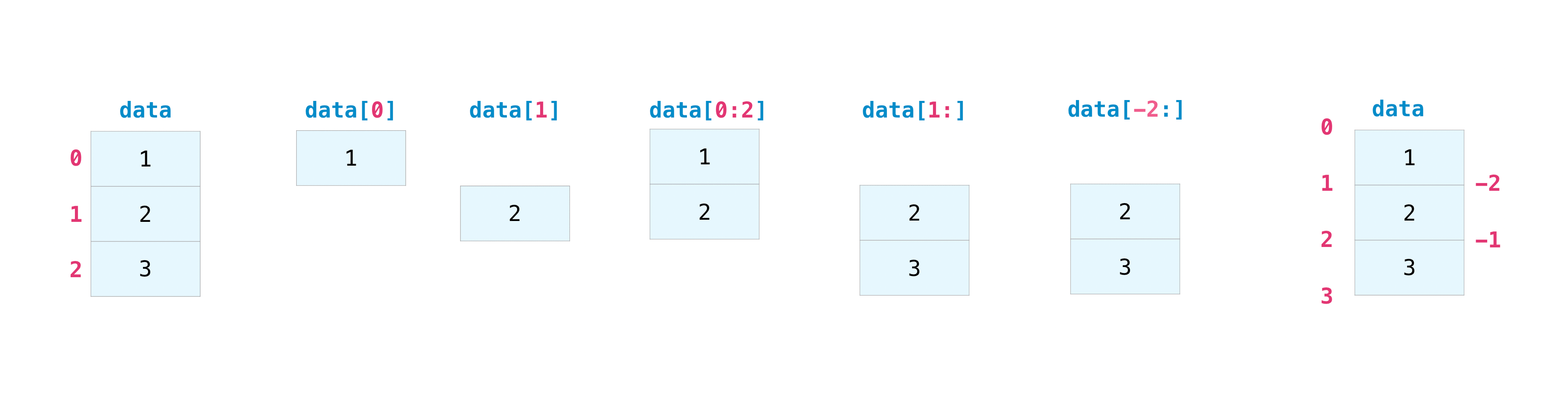

You may need to extract parts of an array or specific elements of an array for further analysis or manipulation. To do this, you will have to subset, slice, and / or index the array.

If you want to extract values from an array that meet certain conditions, NumPy is easy.

For example, take the following array as an example.

>>> a = np.array([[1 , 2, 3, 4], [5, 6, 7, 8], [9, 10, 11, 12]])

You can easily display the numbers less than 5 in the array.

>>> print(a[a < 5])
[1 2 3 4]

You can also, for example, select a number of 5 or greater and use that condition to index the array.

>>> five_up = (a >= 5)
>>> print(a[five_up])
[ 5  6  7  8  9 10 11 12]

You can also extract elements that are divisible by 2. ::

>>> divisible_by_2 = a[a%2==0]
>>> print(divisible_by_2)
[ 2  4  6  8 10 12]

You can also use the & and | operators to retrieve elements that meet two conditions:

>>> c = a[(a > 2) & (a < 11)]
>>> print(c)
[ 3  4  5  6  7  8  9 10]

You can also use the logical operators ** & ** and ** | ** to return a Boolean value that indicates whether the value of the array meets certain conditions. This is useful for arrays with names or values in different categories.

>>> five_up = (a > 5) | (a == 5)
>>> print(five_up)
[[False False False False]
 [ True  True  True  True]
 [ True  True  True True]]

You can also use np.nonzero () to select an element or index from an array. Let's start with the following array:

>>> a = np.array([[1, 2, 3, 4], [5, 6, 7, 8], [9, 10, 11, 12]])

You can use np.nonzero () to display the index of an element, less than 5 in this case:

>>> b = np.nonzero(a < 5)
>>> print(b)
(array([0, 0, 0, 0]), array([0, 1, 2, 3]))

This example returns a tuple of arrays. Only one tuple is returned for each dimension. The first array shows the row indexes that have values that meet the conditions, and the second array shows the column indexes that have the values that meet the conditions.

If you want to generate a list of coordinates with an element, you can zip this array and iterate over the list of coordinates to display it. For example:

>>> list_of_coordinates= list(zip(b[0], b[1]))

>>> for coord in list_of_coordinates:
...    print(coord)
(0, 0)
(0, 1)
(0, 2)
(0, 3)

You can also use np.nonzero () to display less than 5 elements in the array:

>>> print(a[b])
[1 2 3 4]
```shell

 If the element you are looking for does not exist in the array, the return index array will be empty. For example:

​```shell
>>> not_there = np.nonzero(a == 42)
>>> print(not_there)
(array([], dtype=int64), array([], dtype=int64))

How to create an array from existing data

• This section deals with slicing and indexing,np.vstack (),np.hstack (),np.hsplit (),.view (),copy ()*

You can easily create an array from a part of an existing array. Suppose you have the following array:

>>> a = np.array([1,  2,  3,  4,  5,  6,  7,  8,  9, 10])

You can always create a new array from the array part by specifying the part of the array you want to slice.

>>> arr1 = a[3:8]
>>> arr1
array([4, 5, 6, 7, 8])

Here, the range from index position 3 to index position 8 is specified.

You can concatenate two existing arrays either vertically or horizontally. Suppose you have the following two arrays, ʻa1, ʻa2.

>>> a1 = np.array([[1, 1],
...               [2, 2]])

>>> a2 = np.array([[3, 3],
...               [4, 4]])

You can stack these vertically using vstack.

>>> np.vstack((a1, a2))
array([[1, 1],
       [2, 2],
       [3, 3],
       [4, 4]])

And you can stack them side by side with hstack.

>>> np.hstack((a1, a2))
array([[1, 1, 3, 3],
       [2, 2, 4, 4]])

You can split the array into several smaller arrays with hsplit. You can specify how many isomorphic arrays the array will be divided into and the number of columns after the division.

Let's say you have this array:

>>> x = np.arange(1, 25).reshape(2, 12)
>>> x
array([[ 1,  2,  3,  4,  5,  6,  7,  8,  9, 10, 11, 12],
       [13, 14, 15, 16, 17, 18, 19, 20, 21, 22, 23, 24]])

If you want to split this array into three identically shaped arrays, run the following code.

>>> np.hsplit(x, 3)
[array([[1,  2,  3,  4],
        [13, 14, 15, 16]]), array([[ 5,  6,  7,  8],
        [17, 18, 19, 20]]), array([[ 9, 10, 11, 12],
        [21, 22, 23, 24]])]

If you want to split the array after the 3rd and 4th columns, run the following code.

>>> np.hsplit(x, (3, 4))
[array([[1, 2, 3],
        [13, 14, 15]]), array([[ 4],
        [16]]), array([[ 5, 6, 7, 8, 9, 10, 11, 12],
        [17, 18, 19, 20, 21, 22, 23, 24]])]

Learn more about stacking and splitting arrays here.

You can use the view method to create a new array that references the same data as the original array (shallow copy).

Views are one of the key concepts in NumPy. NumPy functions return views as much as possible, similar to operations such as subscript access and slicing. This saves memory and is fast (no need to make a copy of the data). But there is one thing to keep in mind – – changing the data in the view will change the original array as well.

Suppose you create an array like this:

>>> a = np.array([[1, 2, 3, 4], [5, 6, 7, 8], [9, 10, 11, 12]])

Now slice ʻa to make b1and change the first element ofb1. This operation also changes the corresponding element of ʻa.

>>> b1 = a[0, :]
>>> b1
array([1, 2, 3, 4])
>>> b1[0] = 99
>>> b1
array([99,  2,  3,  4])
>>> a
array([[99,  2,  3,  4],
       [ 5,  6,  7,  8],
       [ 9, 10, 11, 12]])

Use the copy method to make a complete copy of the array and its data (deep copy). To use this for an array, run the following code.

>>> b2 = a.copy()

Basic operation of an array

• This section deals with addition, subtraction, multiplication, division, etc. *

Once you've created the array, you can start working on it. For example, let's say you have created two arrays called "data" and "ones".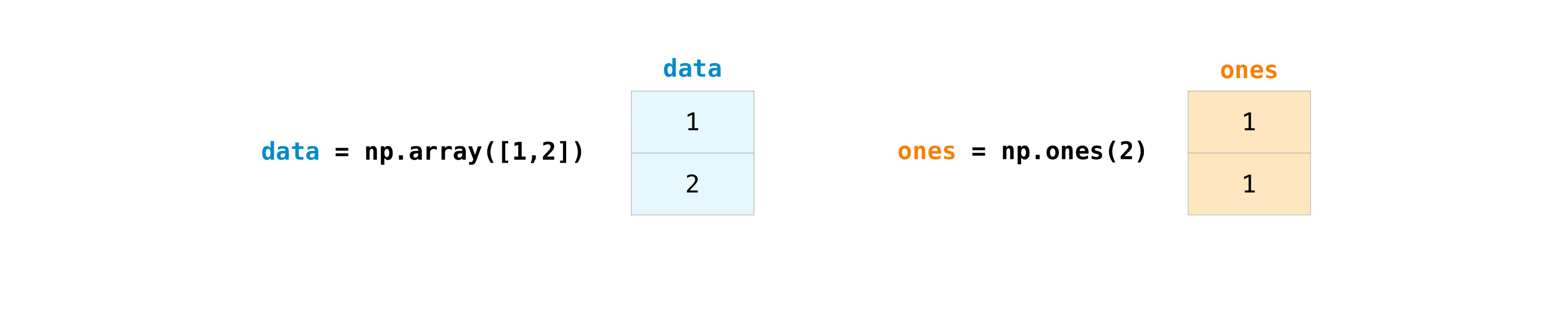

You can add arrays using the plus sign.

>>> data = np.array([1, 2])
>>> ones = np.ones(2, dtype=int)
>>> data + ones
array([2, 3])

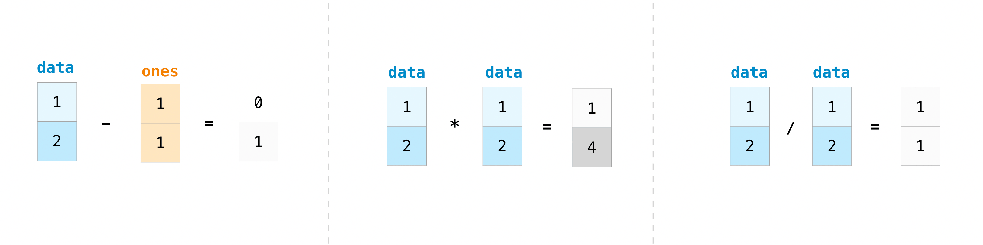
Of course, you can do more than just add!

>>> data - ones
array([0, 1])
>>> data * data
array([1, 4])
>>> data / data
array([1., 1.])

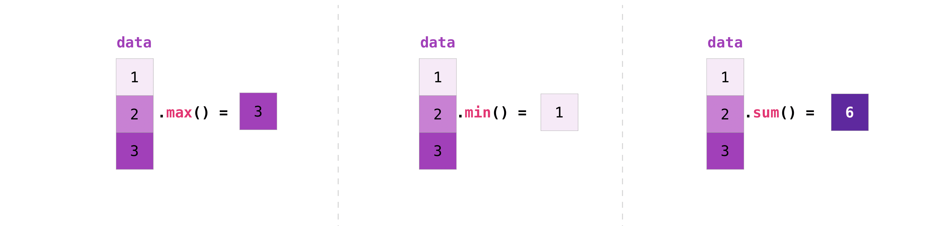
Basic operations are easy with NumPy. If you want to know the sum of the arrays, use sum (). It works in 1D, 2D and above arrays.

>>> a = np.array([1, 2, 3, 4])

>>> a.sum()
10

If you want to add columns or rows in a 2D array (To add the rows or the columns in a 2D array), specify the axes. If you start with this array:

>>> b = np.array([[1, 1], [2, 2]])

The rows can be summed as follows:

>>> b.sum(axis=0)
array([3, 3])

The columns can be summed as follows: ::

>>> b.sum(axis=1)
array([2, 4])

Broadcasting

There are times when you want to perform an operation between an array and a single number, or between arrays of different sizes (the former is also called an operation between a vector and a scalar). For example, suppose an array (called "data") has information about how many miles it is apart and you want to convert it to kilometers. You can do this as follows:

>>> data = np.array([1.0, 2.0])
>>> data * 1.6
array([1.6, 3.2])

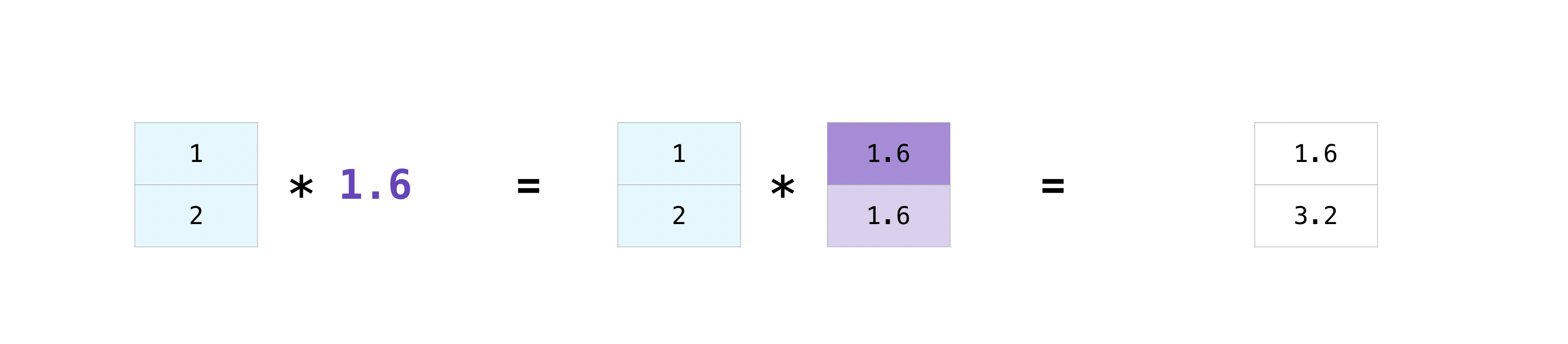
NumPy understands that multiplication must be done in every single cell. This concept is called ** broadcast **. Broadcastet is a mechanism for NumPy to perform operations on arrays of different shapes. The dimensions of the array must be compatible. For example, if both arrays have the same dimension or one is one-dimensional. If not, you will get a ValueError.

More convenient array operations

This section covers maximum, minimum, sum, mean, product, standard deviation, and more

NumPy also executes aggregate functions. In addition to min, max, sum, mean to get the mean, prod to get the result of multiplying the elements, std to get the standard deviation, etc. are easy. Can be executed.

>>> data.max()
2.0
>>> data.min()
1.0
>>> data.sum()
3.0

Let's start with this array, “a”

>>> a = np.array([[0.45053314, 0.17296777, 0.34376245, 0.5510652],
...              [0.54627315, 0.05093587, 0.40067661, 0.55645993],
...              [0.12697628, 0.82485143, 0.26590556, 0.56917101]])

It's very common to want to aggregate along rows and columns. By default, all NumPy aggregate functions return the sum of the entire array. If you want to know the sum or minimum value of the elements of an array, use the following code.

>>> a.sum()
4.8595784

Or:

>>> a.min()
0.05093587

You can specify on which axis you want the aggregate function to work. For example, you can find the minimum value in each column by setting axis = 0.

>>> a.min(axis=0)
array([0.12697628, 0.05093587, 0.26590556, 0.5510652 ])

The above four numbers match the numbers in the rows of the original array. With a four-row array, you can get four values as a result.

Make a line

You can pass a Python list and use NumPy to create a 2D array (or "matrix") that represents that array.

>>> data = np.array([[1, 2], [3, 4]])
>>> data
array([[1, 2],
       [3, 4]])

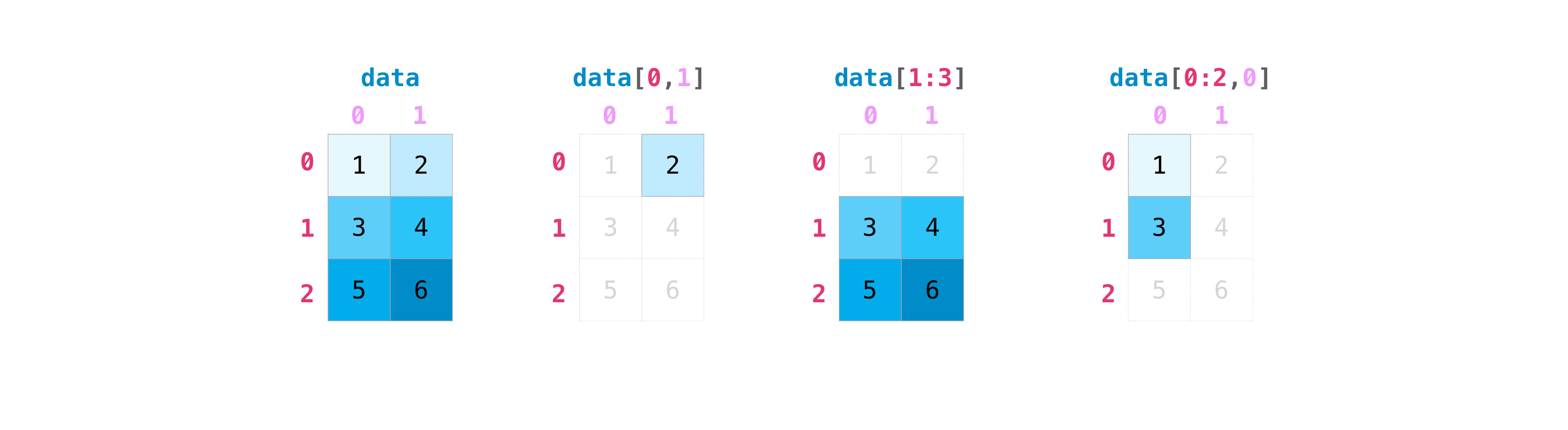
Subscript access and slicing operations are useful when working with matrices.

>>> data[0, 1]
2
>>> data[1:3]
array([[3, 4]])
>>> data[0:2, 0]
array([1, 3])

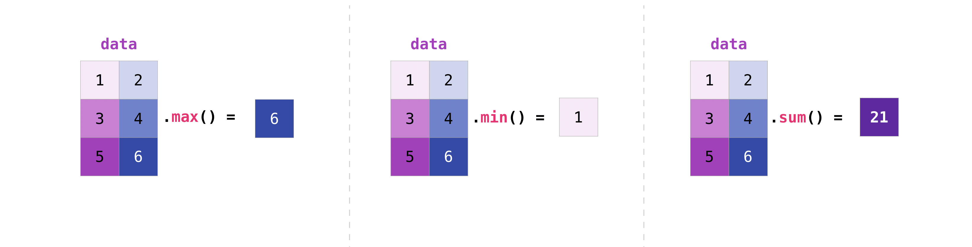
You can work with matrices in the same way you work with vectors.

>>> data.max()
4
>>> data.min()
1
>>> data.sum()
10

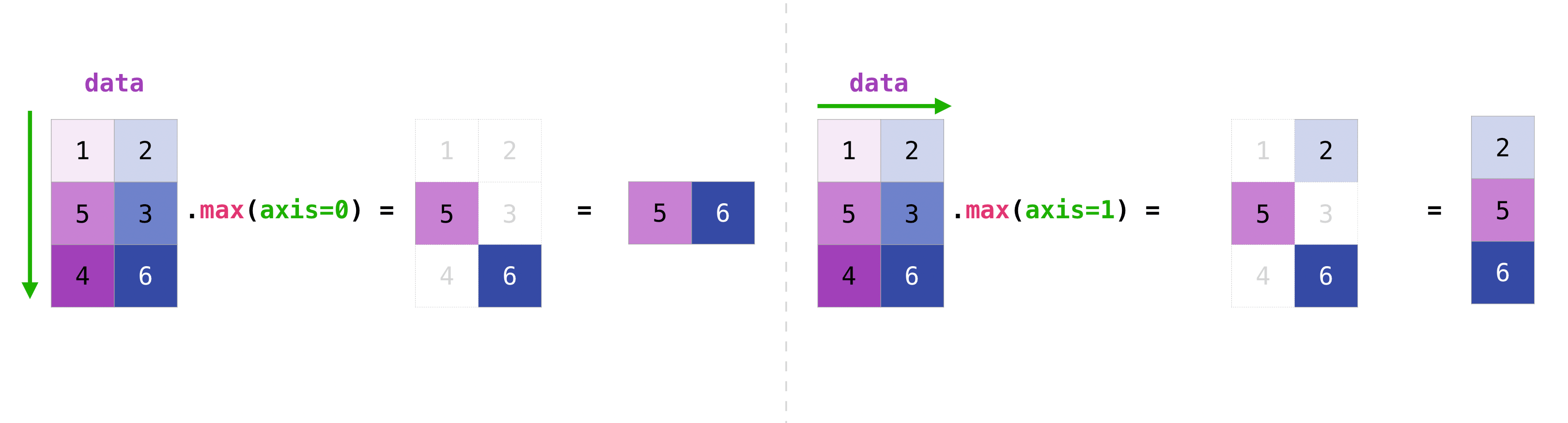
You can aggregate all the values in a matrix, or you can use axis parameters to aggregate across columns or rows.

>>> data.max(axis=0)
array([3, 4])
>>> data.max(axis=1)
array([2, 4])

Once you have created a matrix, if you have two matrices of the same size, you can use arithmetic operators to add and multiply.

>>> data = np.array([[1, 2], [3, 4]])
>>> ones = np.array([[1, 1], [1, 1]])
>>> data + ones
array([[2, 3],
       [4, 5]])

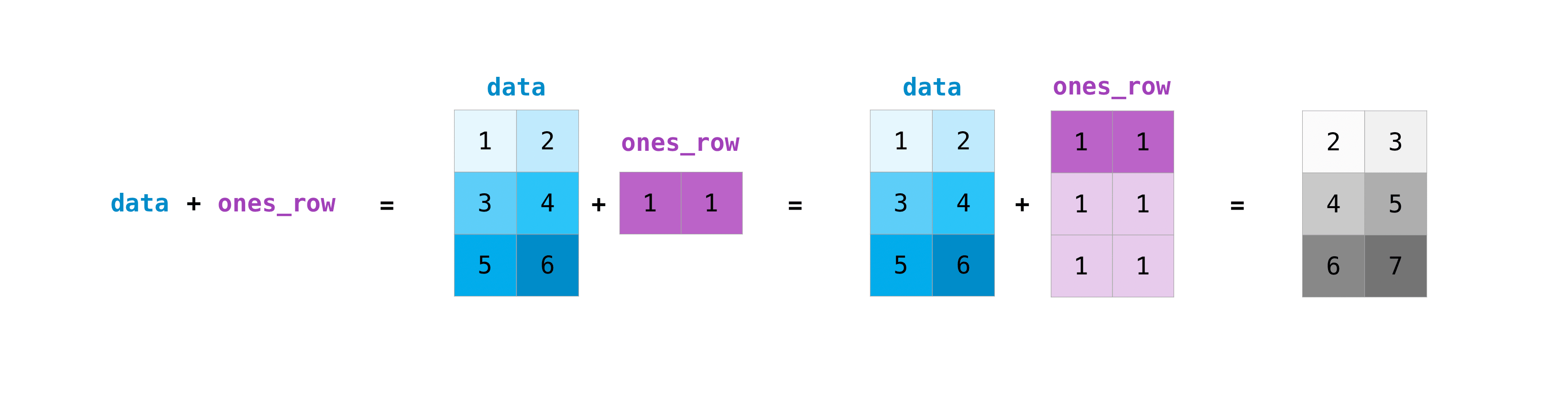
You can perform these arithmetic operations on matrices of different sizes, but only if one matrix has only one row or one column. In this case, NumPy uses broadcast rules for the operation.

>>> data = np.array([[1, 2], [3, 4], [5, 6]])
>>> ones_row = np.array([[1, 1]])
>>> data + ones_row
array([[2, 3],
       [4, 5],
       [6, 7]])

Note that when NumPy displays an N-dimensional array, the last axis loops the most, while the first axis loops loosely [12 times for the column, which is the last axis in the following example. There are 4 loops on the first axis]. For example

>>> np.ones((4, 3, 2))
array([[[1., 1.],
        [1., 1.],
        [1., 1.]],
 
       [[1., 1.],
        [1., 1.],
        [1., 1.]],
 
       [[1., 1.],
        [1., 1.],
        [1., 1.]],
 
       [[1., 1.],
        [1., 1.],
        [1., 1.]]])

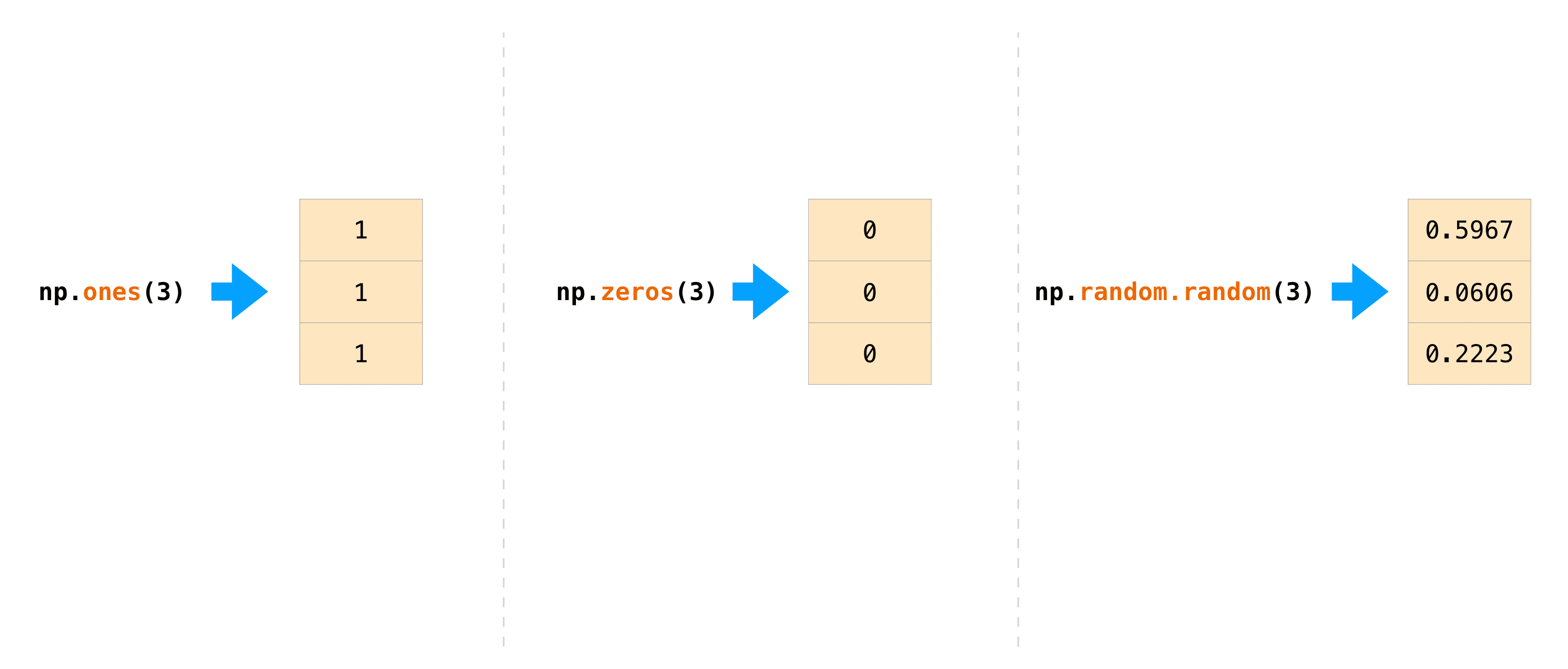
Often you want to initialize an array with NumPy. NumPy provides functions such as ʻones ()andzeros (), as well as the random.Generator` class for random number generation. All you need to do for initialization is pass in the number of elements you want to generate.

>>>np.ones(3)
array([1., 1., 1.])
>>> np.zeros(3)
array([0., 0., 0.])
# the simplest way to generate random numbers
>>> rng = np.random.default_rng(0)
>>> rng.random(3)
array([0.63696169, 0.26978671, 0.04097352])

この関数やメソッドに二次元の行列を表すタプルを与えれば、ones()、zeros()とrandom() を使って二次元配列も生成可能です。

>>> np.ones((3, 2))
array([[1., 1.],
       [1., 1.],
       [1., 1.]])
>>> np.zeros((3, 2))
array([[0., 0.],
       [0., 0.],
       [0., 0.]])
>>> rng.random((3, 2))
array([[0.01652764, 0.81327024],
       [0.91275558, 0.60663578],
       [0.72949656, 0.54362499]])  # may vary

Generate random numbers

The use of random number generators is an important part of the placement and evaluation of many mathematical or machine learning algorithms. Random initialization of the weight of the artificial neural network, division into random sets, or random shuffle of datasets, in any case, is lacking in the ability to generate random numbers (actually, the number of reproducible pseudo-random numbers). I can't. You can use Generator.integers to output a random integer from the minimum to the maximum (note that Numpy includes the minimum and not the maximum). You can set ʻendpoint = True` to generate a random number containing the highest value.

You can generate a 2x4 matrix consisting of random integers from 0 to 4:

>>> rng.integers(5, size=(2, 4))
array([[2, 1, 1, 0],
       [0, 0, 0, 4]])  # may vary

How to retrieve and count non-overlapping elements

• This section deals with np.unique () *

With Np.unique, you can retrieve the elements of an array one by one without duplication. Take this array as an example.

>>> a = np.array([11, 11, 12, 13, 14, 15, 16, 17, 12, 13, 11, 14, 18, 19, 20])

You can use Np.unique to find out the unique values in the array.

>>>
>>> unique_values = np.unique(a)
>>> print(unique_values)
[11 12 13 14 15 16 17 18 19 20]

To get an index of the unique values of a Numpy array (the first index of each unique value of the array), pass the return_index argument tonp.unique ()with the array.

>>> unique_values, indices_list = np.unique(a, return_index=True)
>>> print(indices_list)
[ 0  2  3  4  5  6  7 12 13 14]

You can pass the return_counts argument tonp.unique ()together with the array to see how many unique values each Numpy array has.

>>> unique_values, occurrence_count = np.unique(a, return_counts=True)
>>> print(occurrence_count)
[3 2 2 2 1 1 1 1 1 1]

This also works for 2D arrays! With this array,

>>> a_2d = np.array([[1, 2, 3, 4], [5, 6, 7, 8], [9, 10, 11, 12], [1, 2, 3, 4]])

This way you can find unique values.

>>> unique_values = np.unique(a_2d)
>>> print(unique_values)
[ 1  2  3  4  5  6  7  8  9 10 11 12]

If no axis arguments are passed, the 2D array will be flattened to 1D. If you want to know a unique row or column, be sure to pass the axis argument. Specify ʻaxis = 0 for unique rows and ʻaxis = 1 for columns.

>>> unique_rows = np.unique(a_2d, axis=0)
>>> print(unique_rows)
[[ 1  2  3  4]
 [ 5  6  7  8]
 [ 9 10 11 12]]

To get a unique column, index position and number of occurrences:

>>> unique_rows, indices, occurrence_count = np.unique(
...     a_2d, axis=0, return_counts=True, return_index=True)
>>> print(unique_rows)
[[ 1  2  3  4]
 [ 5  6  7  8]
 [ 9 10 11 12]]
>>> print(indices)
[0 1 2]
>>> print(occurrence_count)
[2 1 1]

Transpose and transformation of matrix

• This section deals with ʻarr.reshape () , ʻarr.transpose (), ʻarr.T () * Matrix transpose is often required. Numpy arrays have the property T` to transpose a matrix.

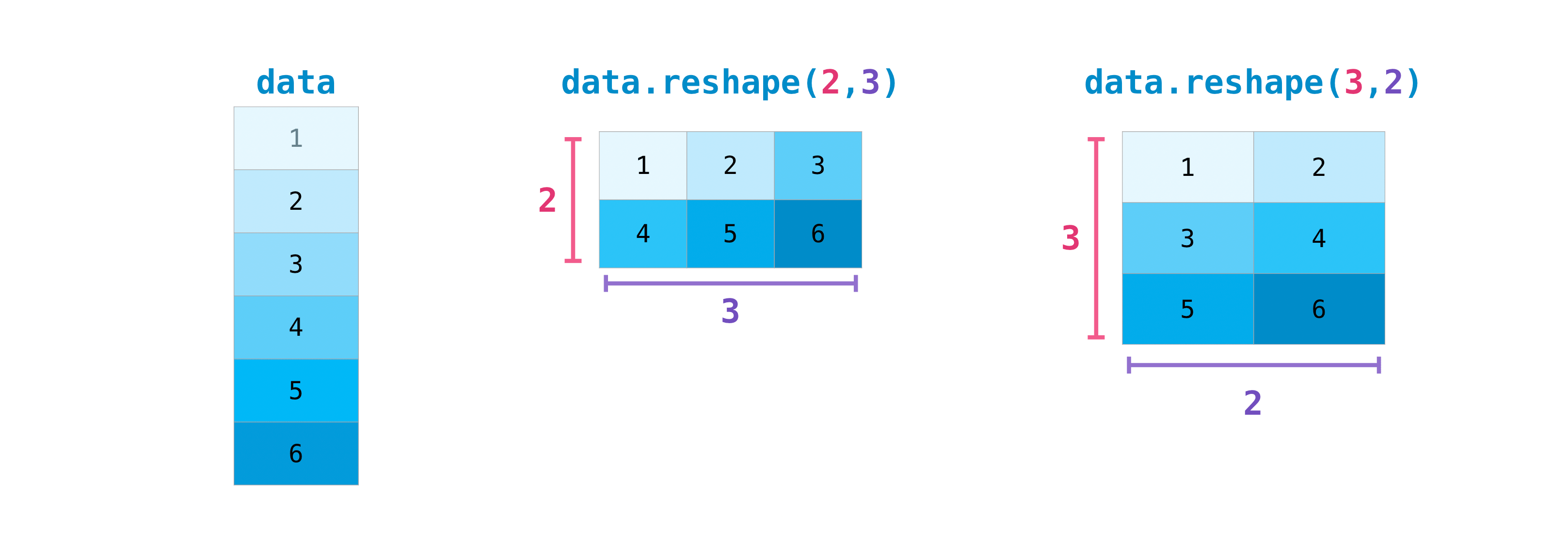
You may also need to swap the dimensions of the array. This happens, for example, if you have a model that assumes an array of inputs that is different from the dataset. The reshape method is useful in such cases. All you need to do is pass the new dimensions [dimensions] you want for the matrix.

>>> data.reshape(2, 3)
array([[1, 2, 3],
       [4, 5, 6]])
>>> data.reshape(3, 2)
array([[1, 2],
       [3, 4],
       [5, 6]])

You can also use .transpose to invert or change the axes of the array according to the values you specify.

Take this array as an example:

>>> arr = np.arange(6).reshape((2, 3))
>>> arr
array([[0, 1, 2],
       [3, 4, 5]])

You can transpose an array using ʻarr.transpose () `.

>>> arr.transpose()
array([[0, 3],
       [1, 4],
       [2, 5]])

How to invert an array

• This section deals with np.flip *

NumPy's np.flip () can flip the axis of an array relative to axis. When using np.flip (), specify the array and axis you want to flip. If you don't specify an axis, NumPy inverts the given array for all axes.

Invert 1D array

Take the following one-dimensional array as an example:

>>> arr = np.array([1, 2, 3, 4, 5, 6, 7, 8])

You can invert the array this way:

>>> reversed_arr = np.flip(arr)

If you want to see the inverted array, run this code:

>>> print('Reversed Array: ', reversed_arr)
Reversed Array:  [8 7 6 5 4 3 2 1]

Invert 2D array

2D arrays are flipped in much the same way.

Take this array as an example:

>>> arr_2d = np.array([[1, 2, 3, 4], [5, 6, 7, 8], [9, 10, 11, 12]])

You can invert the contents on all columns and rows.

>>> reversed_arr = np.flip(arr_2d)
>>> print(reversed_arr)
[[12 11 10  9]
 [ 8  7  6  5]
 [ 4  3  2  1]]

This is the only way to invert lines only:

>>> reversed_arr_rows = np.flip(arr_2d, axis=0)
>>> print(reversed_arr_rows)
[[ 9 10 11 12]
 [ 5  6  7  8]
 [ 1  2  3  4]]

To flip just the columns:

>>> reversed_arr_columns = np.flip(arr_2d, axis=1)
>>> print(reversed_arr_columns)
[[ 4  3  2  1]
 [ 8  7  6  5]
 [12 11 10  9]]

You can also invert just one row or column. For example, you can invert the row with index 1 (second row):

>>> arr_2d[1] = np.flip(arr_2d[1])
>>> print(arr_2d)
[[ 1  2  3  4]
 [ 8  7  6  5]
 [ 9 10 11 12]]

You can also invert the column with index 1 (second column):

>>> arr_2d[:,1] = np.flip(arr_2d[:,1])
>>> print(arr_2d)
[[ 1 10  3  4]
 [ 8  7  6  5]
 [ 9  2 11 12]]

How to reshape and flatten a multidimensional array

• This section deals with .flatten (), ravel () *

There are two common ways to flatten an array. .flatten () and .ravel (). The main difference between the two is that the array created using .ravel () is actually a reference (or "view") to the parent array. So if you change anything in the new array, the parent array will change as well. ravel does not make a copy, so it is memory efficient.

>>> x = np.array([[1 , 2, 3, 4], [5, 6, 7, 8], [9, 10, 11, 12]])

You can use flatten to make an array a 1D array.

>>> x.flatten()
array([ 1,  2,  3,  4,  5,  6,  7,  8,  9, 10, 11, 12])

With flatten', changes to the array are not applied to the parent array.

For example:

>>> a1 = x.flatten()
>>> a1[0] = 99
>>> print(x)  # Original array
[[ 1  2  3  4]
 [ 5  6  7  8]
 [ 9 10 11 12]]
>>> print(a1)  # New array
[99  2  3  4  5  6  7  8  9 10 11 12]

But with ravel, changes to the array are not applied to the parent array.

>>> a2 = x.ravel()
>>> a2[0] = 98
>>> print(x)  # Original array
[[98  2  3  4]
 [ 5  6  7  8]
 [ 9 10 11 12]]
>>> print(a2)  # New array
[98  2  3  4  5  6  7  8  9 10 11 12]

Visit the docstring to find out more

This section deals with help (), ?, ??.

When it comes to the data science ecosystem, Python and NumPy are built with the user in mind. One good example of this is that it has access to the documentation. Every object has a reference to a string, which we know as a docstring. In most cases, this docstring contains a brief and concise overview of the object and how to use it. Python has a built-in help function, which helps you access the docstring. This means that when you need more information, you can usually use help () to quickly find the information you need.

For example

>>> help(max)
Help on built-in function max in module builtins:
 
max(...)
    max(iterable, *[, default=obj, key=func]) -> value
    max(arg1, arg2, *args, *[, key=func]) -> value
 
    With a single iterable argument, return its biggest item. The
    default keyword-only argument specifies an object to return if
    the provided iterable is empty.
    With two or more arguments, return the largest argument.

Access to more information can be quite helpful, so what about IPython? Is used as an abbreviation to access other information related to the documentation. IPython is a command shell for interactive calculations that can be used in multiple languages. Learn more about IPython.

For example

In [0]: max?
max(iterable, *[, default=obj, key=func]) -> value
max(arg1, arg2, *args, *[, key=func]) -> value
 
With a single iterable argument, return its biggest item. The
default keyword-only argument specifies an object to return if
the provided iterable is empty.
With two or more arguments, return the largest argument.
Type:      builtin_function_or_method

You can even use this notation for object methods and even the objects themselves.

Let's say you have created the following array.

>>> a = np.array([1, 2, 3, 4, 5, 6])

This will give you a lot of useful information (first the details of the object itself, followed by the docstring of the ndarray where a is an instance).

In [1]: a?
Type:            ndarray
String form:     [1 2 3 4 5 6]
Length:          6
File:            ~/anaconda3/lib/python3.7/site-packages/numpy/__init__.py
Docstring:       <no docstring>
Class docstring:
ndarray(shape, dtype=float, buffer=None, offset=0,
        strides=None, order=None)
 
An array object represents a multidimensional, homogeneous array
of fixed-size items.  An associated data-type object describes the
format of each element in the array (its byte-order, how many bytes it
occupies in memory, whether it is an integer, a floating point number,
or something else, etc.)
 
Arrays should be constructed using `array`, `zeros` or `empty` (refer
to the See Also section below).  The parameters given here refer to
a low-level method (`ndarray(...)`) for instantiating an array.
 
For more information, refer to the `numpy` module and examine the
methods and attributes of an array.
 
Parameters
----------
(for the __new__ method; see Notes below)
 
shape : tuple of ints
        Shape of created array.
...

This also works for functions and other objects you create. However. Don't forget to put the docstring inside the function using character literals (enclose the documentation in " "" "" " or ''''''').

For example, if you create the following function

>>> def double(a):
...  '''Return a * 2'''
...  return a * 2

To get information about this function:

 In [2]: double?
Signature: double(a)
Docstring: Return a * 2
File:      ~/Desktop/<ipython-input-23-b5adf20be596>
Type:      function

You can get a different level of information by reading the source code of the object you are interested in. You can access the source code by using a double question mark (??).

For example

In [3]: double??
Signature: double(a)
Source:
def double(a):
    '''Return a * 2'''
    return a * 2
File:      ~/Desktop/<ipython-input-23-b5adf20be596>
Type:      function

If the object is compiled in a language other than Python, using ?? will return the same information as ?. This can be seen in many built-in objects and types. For example

In [4]: len?
Signature: len(obj, /)
Docstring: Return the number of items in a container.
Type:      builtin_function_or_method

And:

In [5]: len??
Signature: len(obj, /)
Docstring: Return the number of items in a container.
Type:      builtin_function_or_method

They have the same output because they are compiled in a language other than Python.

Handle mathematical formulas

One of the reasons NumPy is so popular in the Python community of science is that it's easy to implement mathematical formulas that work on arrays.

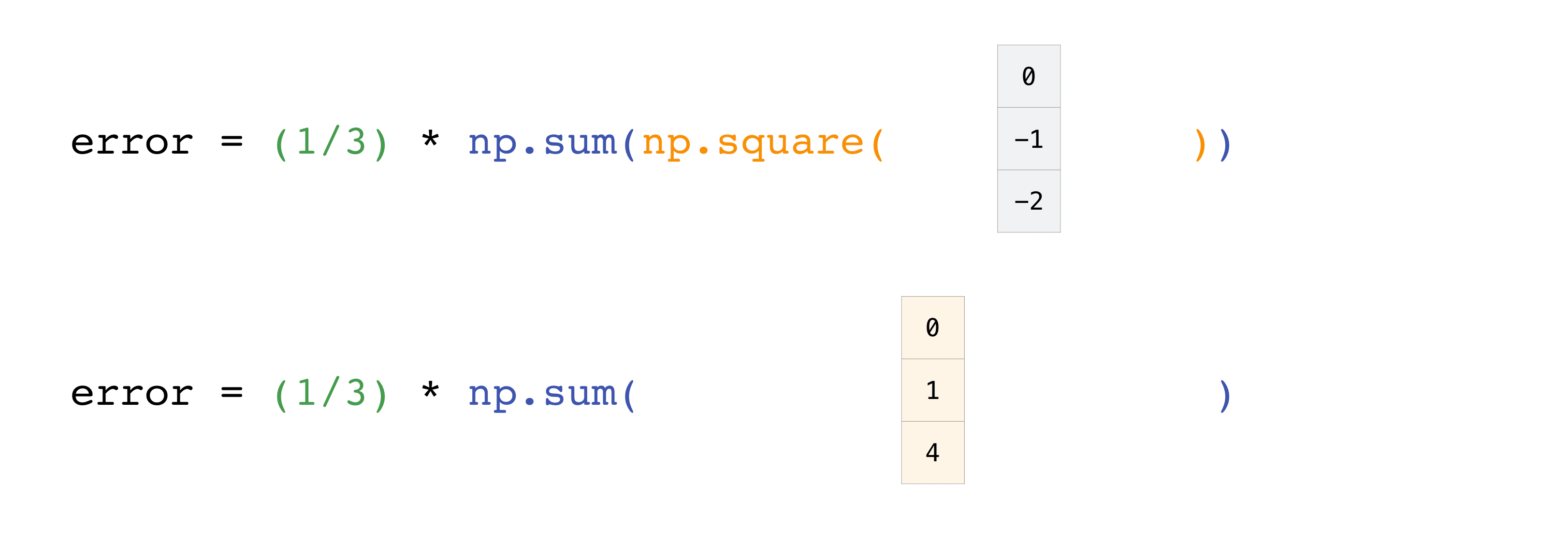
For example, this is the mean square error, the central formula used in supervised machine learning models that deal with regression.

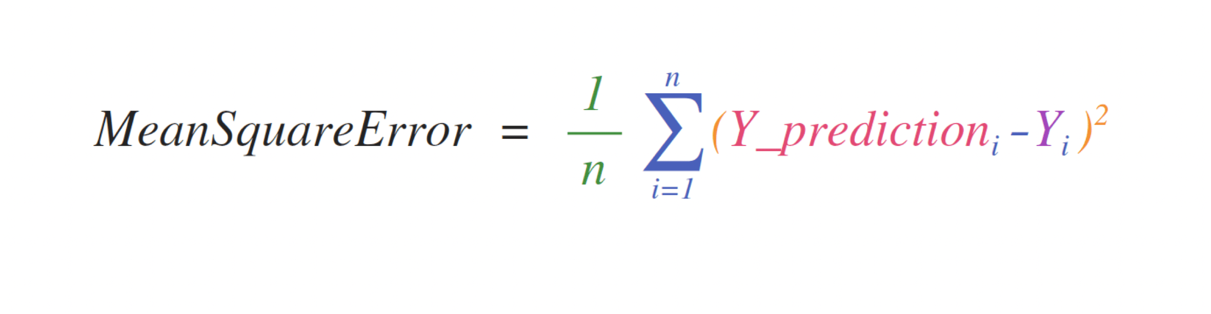
The implementation of this expression is simple in NumPy and is the same as the expression:

error  = (1/n) * np.sum(np.square(predictions - labels))

This works very well because it can contain either one or 1000 predicted values and labels. All you need is that the predicted value and the label are the same size.

This can be visualized as follows:

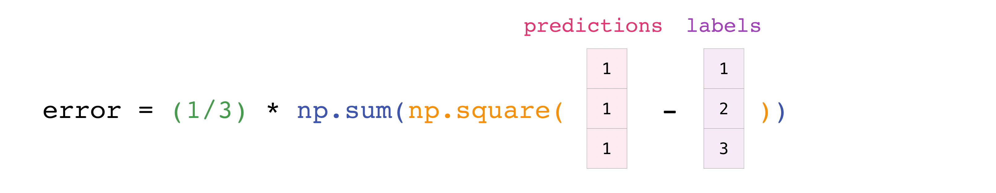
In this example, the prediction and label are Bertholds with three values, so n takes the value 3. After the subtraction, the vector value is squared. NumPy then sums the values, and the result is a score of predicted error and model quality.

How to save and load NumPy

• This section deals with np.save, np.savez, np.savetxt, np.load, np.loadtxt *

At some point you may want to save the array to disk and load it without having to run the code again. Fortunately, NumPy has several ways to save and load objects. The ndarray object can load and save regular text files with the loadtxt and savetxt functions, and handle NumPy binary files with a .npz extension with the load and save functions. You can then use the savez function to work with Numpy files with a .npz extension.

The **. npy ** and **. npz ** files store data, shape, dtype and other information needed to rebuild the ndarray so that the files can be recovered correctly on different architectures. I am.

If you want to save one ndarray object, use np.save to save it as a .npy file. If you want to save multiple ndarrays in an array, use np.savez and save as .npz. You can also save multiple arrays in one file by saving them in npz format compressed with savez_compressed.

It ’s easy to save and load and array with np.save (). Don't forget to specify the array and file name you want to save. For example, if you create this array

>>> a = np.array([1, 2, 3, 4, 5, 6])

You can save it as "filename.npy".

>>> np.save('filename', a)

You can restore the array with np.load ().

>>> b = np.load('filename.npy')

If you want to see the array, you can run this code.

>>> print(b)
[1 2 3 4 5 6]

You can use np.savetxt to save NumPy files as plain text like .csv and .txt files.

For example, if you create the following array

>>> csv_arr = np.array([1, 2, 3, 4, 5, 6, 7, 8])
​```shell
 
You can easily save it as a .csv file with the name “new_file.csv” like this:

​```shell
>>> np.savetxt('new_file.csv', csv_arr)

You can easily load a saved text file using loadtxt ().

>>> np.loadtxt('new_file.csv')
array([1., 2., 3., 4., 5., 6., 7., 8.])

The savetxt () and loadtxt () functions accept additional parameters such as headers, footers, and delimiters. Text files are convenient for sharing, while .npy and .npz files are small and fast to read and write. If you need more sophisticated handling of text files (for example, when dealing with matrices [lines] containing missing values), genfromtxt You will need to use the .genfromtxt.html # numpy.genfromtxt) function.

When using savetxt, you can specify headers, footers, comments, etc.

Learn more about input and output routines here.

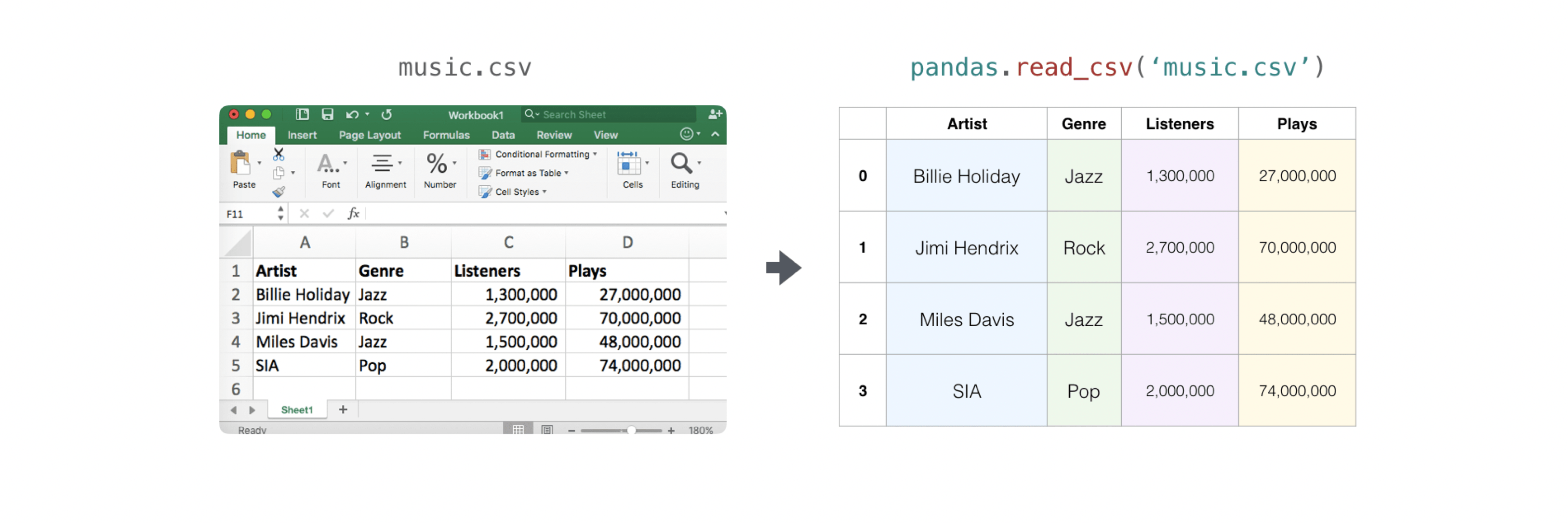
How to import / export CSV

It's easy to read a CSV file that contains existing information. The easiest way is to use Pandas.

>>> import pandas as pd
 
>>> # If all of your columns are the same type:
>>> x = pd.read_csv('music.csv', header=0).values
>>> print(x)
[['Billie Holiday' 'Jazz' 1300000 27000000]
 ['Jimmie Hendrix' 'Rock' 2700000 70000000]
 ['Miles Davis' 'Jazz' 1500000 48000000]
 ['SIA' 'Pop' 2000000 74000000]]
 
>>> # You can also simply select the columns you need:
>>> x = pd.read_csv('music.csv', usecols=['Artist', 'Plays']).values
>>> print(x)
[['Billie Holiday' 27000000]
 ['Jimmie Hendrix' 70000000]
 ['Miles Davis' 48000000]
 ['SIA' 74000000]]

Exporting an array is also easy with Pandas. If you're new to NumPy, it's a good idea to create a Pandas dataframe from array values and write that dataframe to a CSV file with Pandas.

Let's say you have created the array "a".

>>> a = np.array([[-2.58289208,  0.43014843, -1.24082018, 1.59572603],
...              [ 0.99027828, 1.17150989,  0.94125714, -0.14692469],
...              [ 0.76989341,  0.81299683, -0.95068423, 0.11769564],
...              [ 0.20484034,  0.34784527,  1.96979195, 0.51992837]])

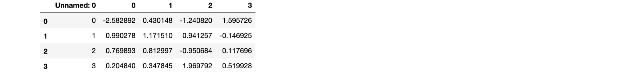
You can create a Pandas data frame as follows:

>>> df = pd.DataFrame(a)
>>> print(df)
          0         1         2         3
0 -2.582892  0.430148 -1.240820  1.595726
1  0.990278  1.171510  0.941257 -0.146925
2  0.769893  0.812997 -0.950684  0.117696
3  0.204840  0.347845  1.969792  0.519928

You can save the data frame as follows:

>>> df.to_csv('pd.csv')

CSV is like this

>>> data = pd.read_csv('pd.csv')

NumPyのsavetxtメソッドを使って保存することもできます。

>>> np.savetxt('np.csv', a, fmt='%.2f', delimiter=',', header='1,  2,  3,  4')

If you are using the command line, you can always load the CSV saved with a command like this:

$ cat np.csv
#  1,  2,  3,  4
-2.58,0.43,-1.24,1.60
0.99,1.17,0.94,-0.15
0.77,0.81,-0.95,0.12
0.20,0.35,1.97,0.52

Alternatively, you can open it in a text editor at any time.

If you want to know more about Pandas, take a look at the official Pandas documentation. See official Pandas installation information for instructions on how to install Pandas.

Plot the array with Matplotlib

If you need to create a plot of values, Matplotlib is very easy to use.

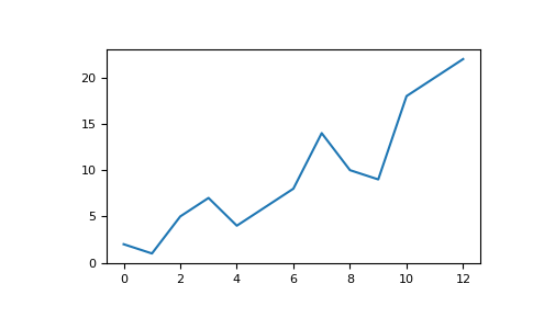
For example, you might have an array like this:

>>> a = np.array([2, 1, 5, 7, 4, 6, 8, 14, 10, 9, 18, 20, 22])

If you already have Matplotlib installed, you can import it like this:

>>> import matplotlib.pyplot as plt
 
# If you're using Jupyter Notebook, you may also want to run the following
# line of code to display your code in the notebook:
 
%matplotlib inline

No tedious work is required to plot the values.

>>> plt.plot(a)
 
# If you are running from a command line, you may need to do this:
# >>> plt.show()

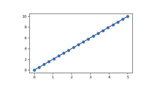
For example, you can plot a 1D array as follows:

‘>>> x = np.linspace(0, 5, 20)
>>> y = np.linspace(0, 10, 20)
>>> plt.plot(x, y, 'purple') # line
>>> plt.plot(x, y, 'o')      # dots

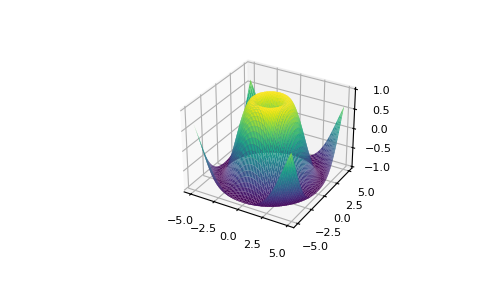
Matplotlib offers a huge number of visualization options.

>>> from mpl_toolkits.mplot3d import Axes3D
>>> fig = plt.figure()
>>> ax = Axes3D(fig)
>>> X = np.arange(-5, 5, 0.15)
>>> Y = np.arange(-5, 5, 0.15)
>>> X, Y = np.meshgrid(X, Y)
>>> R = np.sqrt(X**2 + Y**2)
>>> Z = np.sin(R)
 
>>> ax.plot_surface(X, Y, Z, rstride=1, cstride=1, cmap='viridis')

To read more about Matplotlib and what it can do, take a look at the official documentation.FordirectionsregardinginstallingMatplotlib,seetheofficialinstallationsection.

mage credits: Jay Alammar http://jalammar.github.io/