[PYTHON] [Deprecated] Chainer v1.24.0 Tutorial for beginners

warning

This article is too old to be funny, written for the final release of Chainer v1 (v1.24.0), which is no longer supported.

** There is an article written for the latest stable version of Chainer v3 as of December 2017 at here, so it is absolutely necessary to get started with v1. Unless you have a very special situation, please fly to there now. ** **

Go !!-> Chainer v3 Beginner Tutorial

1st Chainer Beginner's Hands-on was held in the multipurpose room of the Preferred Networks office in Otemachi. This article is an article about what we did in this hands-on.

The materials used on the day of hands-on are summarized in the following Github repository.

mitmul/chainer-handson

On the day of the event, 20 GPU servers equipped with 4 Pascal TITAN X (80 GPUs in total!) Were borrowed from Sakura Internet free of charge and hands-on was held for all participants to use. We would like to take this opportunity to thank Sakura Internet. It is said that Sakura High Thermal Computing will soon start a GPU server rental service on an hourly basis, so if you are considering introducing a GPU environment, please check it out.

Sakura High Thermal Power Computing

On the day of hands-on, I started by ssh logging in to each node of this borrowed Sakura high heat power and installing NVIDIA CUDA, but in this article I skipped that part and summarized from the part on how to use Chainer I will continue.

Please refer to the following materials for how to build the environment.

Environment construction on Sakura high-power computing server

This can be used as a procedure for building an environment for a server running NVIDIA GPU running on Ubuntu 14.04, except for some.

Now let's get into the main subject. The following is a tutorial written assuming Python 3.4, which is installed by default on Ubuntu 14.04. Please refer to P.9 and P.11 of the above document in advance to install the related libraries and Chainer itself. ** The following code part and the output result that follows are assumed to be executed on Jupyter notebook. ** **

Let's write a learning loop

here,

1. Extract data from the dataset
2. Fill in the model
3. Use Optimizer to update model parameters and run a training loop

I will try that. Through these, you can experience how to write a learning loop without using Trainer.

1. Data set preparation

Here, we will use a convenient method for using the MNIST dataset provided by Chainer. With it, everything from downloading data to being able to retrieve individual data is hidden.

from chainer.datasets import mnist

#If the dataset has not been downloaded, download it as well
train, test = mnist.get_mnist(withlabel=True, ndim=1)

#Makes the graph drawing result using matplotlib displayed in the notebook.
%matplotlib inline
import matplotlib.pyplot as plt

#Data example
x, t = train[0]
plt.imshow(x.reshape(28, 28), cmap='gray')
plt.show()
print('label:', t)

Output result:

Downloading from http://yann.lecun.com/exdb/mnist/train-images-idx3-ubyte.gz...
Downloading from http://yann.lecun.com/exdb/mnist/train-labels-idx1-ubyte.gz...
Downloading from http://yann.lecun.com/exdb/mnist/t10k-images-idx3-ubyte.gz...
Downloading from http://yann.lecun.com/exdb/mnist/t10k-labels-idx1-ubyte.gz...

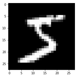
label: 5

2. Creating an Iterator

Let's create a ʻIteratorthat gets a fixed number of data from a dataset and bundles them together to create a mini-batch and return it. We will use this in the learning loop that follows. The iterator will return a new mini-batch with thenext () method. Internally, it has properties (ʻis_new_epoch) that control how many laps the dataset was licked (ʻepoch`) and whether the current iteration is the first iteration of the new epoch.

from chainer import iterators

batchsize = 128

train_iter = iterators.SerialIterator(train, batchsize)
test_iter = iterators.SerialIterator(test, batchsize,
                                     repeat=False, shuffle=False)

About Iterator

--Serial Iterator, which is a kind of Iterator prepared by Chainer, is the simplest Iterator that retrieves the data in the dataset in order. --Take the dataset object and batch size as arguments. --If you need to read the data repeatedly from the dataset object passed at this time for many laps, set the repeat argument to True, and if you do not want to retrieve any more data after one lap, this Let be False. The default is True. --If you pass True to the shuffle` argument, the order of the data retrieved from the dataset will be changed randomly for each epoch.

Here, since batchsize = 128 is set, the train_iter which is the ʻIterator for the training data and the test_iter which is the ʻIterator for the test data created here are 128 numerical image data respectively. Is returned as a batch ʻIterator`. [^ Training data and Validation data]

3. Model definition

Here we define a simple three-layer perceptron. This is a network consisting of only fully connected layers. The number of units in the middle layer is appropriately set to 100, and the output is 10 classes, so set it to 10. This is because the MNIST dataset used here has 10 different labels. Now, let's take a brief look at the Link, Function, and Chain needed to define a model.

Link and Function

--Chainer distinguishes each layer of the neural network into Link and Function. -** Link is a function with parameters. ** ** -** Function is a function with no parameters. ** ** --Combine these to describe the model. --There are many layers with parameters under the chainer.links module. --There are many layers without parameters under the chainer.functions module. --To make these easy to use

import chainer.links as L
import chainer.functions as F

It is customary to give it an alias and use it like L.Convolution2D (...) or F.relu (...).

Chain

--Chain is a class ** for grouping layers with parameters = ** Link. --Having parameters basically means that you need to update them as you train your model (with exceptions). --So, in order to easily get all the parameters that ʻOptimizer should update during learning, we will put them together in one place with Chain`.

Model defined by inheriting Chain

--Models are often defined as classes that inherit from the Chain class. --In that case, in the constructor of the class that represents the model, if you pass the name of the layer you want to register in the form of keyword arguments and the object to the constructor of the parent class, it will be automatically retained in the form found from ʻOptimizer. Will leave it. --This can also be done elsewhere using the ʻadd_link method. --Also, it is convenient to define the __call__ method and describe the forward process in it so that you can pass data to the model with the()accessor like a function call.

To run on GPU

--The Chain class has a to_gpu method, and if you specify a GPU ID in this argument, all the parameters of the model will be transferred to the memory of the specified GPU ID. --This is required to perform forward / backward calculations inside the model on that specified GPU. --If you don't do this, those things will be done on the CPU.

Now let's define the model. First, let's fix the random number seed so that we can reproduce almost the same result as this article. (If you want to guarantee the reproducibility of the calculation result more strictly, you need to know about the option deterministic. This article is useful: Why and the countermeasure that the result changes every time using GPU with Chainer //qiita.com/TokyoMickey/items/cc8cd43545f2656b1cbd).

import numpy
numpy.random.seed(0)
import chainer
if chainer.cuda.available:
    chainer.cuda.cupy.random.seed(0)

Now let's actually define the model, create an object, and send it to the GPU.

import chainer
import chainer.links as L
import chainer.functions as F

class MLP(chainer.Chain):

    def __init__(self, n_mid_units=100, n_out=10):
        #Registration of layers with parameters
        super(MLP, self).__init__(
            l1=L.Linear(None, n_mid_units),
            l2=L.Linear(n_mid_units, n_mid_units),
            l3=L.Linear(n_mid_units, n_out),
        )

    def __call__(self, x):
        #Write forward calculation when data is received
        h1 = F.relu(self.l1(x))
        h2 = F.relu(self.l2(h1))
        return self.l3(h2)

gpu_id = 0

model = MLP()
model.to_gpu(gpu_id)  #Comment out this line if you want the CPU to do the work.

NOTE

Here, the L.Linear class means a fully connected layer. If you pass None as the first argument of the constructor, at runtime, the moment data is input to that layer, the required number of input units will be calculated automatically, and(n_input)$ \ times $ Create a matrix of size n_mid_units and keep it as a parameter. This is a useful feature later, such as when placing the convolution layer in front of the fully connected layer.

As mentioned earlier, Link has a parameter, so you can access the value of that parameter. For example, the model MLP above has a fully connected layer named l1 registered. This fully coupled phase has two parameters, W and b. These can be accessed from the outside. For example, to access b, do the following:

print('The form of the bias parameter of the first fully coupled phase is', model.l1.b.shape)
print('The value immediately after initialization is', model.l1.b.data)

Output result

The form of the bias parameter of the first fully coupled phase is(100,)
The value immediately after initialization is[ 0.  0.  0.  0.  0.  0.  0.  0.  0.  0.  0.  0.  0.  0.  0.  0.  0.  0.
  0.  0.  0.  0.  0.  0.  0.  0.  0.  0.  0.  0.  0.  0.  0.  0.  0.  0.
  0.  0.  0.  0.  0.  0.  0.  0.  0.  0.  0.  0.  0.  0.  0.  0.  0.  0.
  0.  0.  0.  0.  0.  0.  0.  0.  0.  0.  0.  0.  0.  0.  0.  0.  0.  0.
  0.  0.  0.  0.  0.  0.  0.  0.  0.  0.  0.  0.  0.  0.  0.  0.  0.  0.
  0.  0.  0.  0.  0.  0.  0.  0.  0.  0.]

Now, when I try to access model.l1.W, I get the following error:

AttributeError: 'Linear' object has no attribute 'W'

This is because in the definition of the above model, None is passed as the first argument of the constructor of the Linear link, so the matrix W is not allocated until runtime. It does not exist, but it is known inside the Linear object that it will exist.

4. Selection of optimization method

Chainer offers many optimization techniques. They are under the chainer.optimizers module. Here we use ʻoptimizers.SGD, which is the simplest gradient descent method. Pass the model (Chain object) to the Optimizer object using the setup` method. This will allow Optimizer to automatically follow the parameters in the model that it should update.

You can easily try various other optimization methods, so please try them out and see how the results change. For example, in the chainer.optimizers.SGD below, change the SGD part to Momentum SGD, RMSprop, ʻAdam`, etc. and see the difference in the results.

from chainer import optimizers

optimizer = optimizers.SGD(lr=0.01)
optimizer.setup(model)

NOTE

This time I gave $ 0.01 $ to the argument lr in the SGD constructor. This value is known as the learning rate and is known as an important ** hyperparameter ** that needs to be adjusted for good training and good performance of the model.

5. Learning loop

It's finally a learning loop. Since this is a classification problem, we will use the loss function softmax_cross_entropy to calculate the value of the loss that should be minimized.

In Chainer, the forward calculation of the model is performed using Function and Link, the result and the correct answer label are passed to the loss function which is a kind of Function and returns the scalar value, and when the loss is calculated, it is. Like any other Link or Function, it returns a Variable object. Since the Variable object holds a reference to go back to the previous calculation process in the reverse direction, just call theVariable.backward ()method and the calculation from there will be done automatically. It goes back in time and calculates the gradient of the parameters used in the calculations performed along the way.

In other words, the following four items are performed in one learning loop.

1. Pass the data to the model and get the output y
2. Using y and the correct label t, calculate the value of loss to be minimized with the softmax_cross_entropy function.
3. Call the backward method of the output Variable of the softmax_cross_entropy function to give the parameters inside the model the grad property (which is the gradient used to update the parameters).
4. Call the Optimizer's ʻupdate method and update all parameters using the grad` calculated in 3.

that's all. If you are working on a simple regression problem instead of a classification problem, you can use F.mean_squared_error instead of F.softmax_cross_entropy. In addition, Chainer provides various loss functions to handle various problem settings. You can see the list here: Loss functions.

Now, let's write a training loop.

import numpy as np
from chainer.dataset import concat_examples
from chainer.cuda import to_cpu

max_epoch = 10

while train_iter.epoch < max_epoch:
    
    # ----------1 iteration of learning----------
    train_batch = train_iter.next()
    x, t = concat_examples(train_batch, gpu_id)
    
    #Predicted value calculation
    y = model(x)

    #Loss calculation
    loss = F.softmax_cross_entropy(y, t)

    #Gradient calculation
    model.cleargrads()
    loss.backward()

    #Parameter update
    optimizer.update()
    # ---------------So far----------------

    #Measure the prediction accuracy for validation data at the end of each epoch,
    #Let's check that the generalization performance of the model is improved
    if train_iter.is_new_epoch:  #When 1 epoch is over

        #Display of loss
        print('epoch:{:02d} train_loss:{:.04f} '.format(
            train_iter.epoch, float(to_cpu(loss.data))), end='')

        test_losses = []
        test_accuracies = []
        while True:
            test_batch = test_iter.next()
            x_test, t_test = concat_examples(test_batch, gpu_id)

            #Test data forward
            y_test = model(x_test)

            #Calculate loss
            loss_test = F.softmax_cross_entropy(y_test, t_test)
            test_losses.append(to_cpu(loss_test.data))

            #Calculate accuracy
            accuracy = F.accuracy(y_test, t_test)
            accuracy.to_cpu()
            test_accuracies.append(accuracy.data)
            
            if test_iter.is_new_epoch:
                test_iter.epoch = 0
                test_iter.current_position = 0
                test_iter.is_new_epoch = False
                test_iter._pushed_position = None
                break

        print('val_loss:{:.04f} val_accuracy:{:.04f}'.format(
            np.mean(test_losses), np.mean(test_accuracies)))

Output result

epoch:01 train_loss:0.7828 val_loss:0.8276 val_accuracy:0.8167
epoch:02 train_loss:0.3672 val_loss:0.4564 val_accuracy:0.8826
epoch:03 train_loss:0.3069 val_loss:0.3702 val_accuracy:0.8976
epoch:04 train_loss:0.3333 val_loss:0.3307 val_accuracy:0.9078
epoch:05 train_loss:0.3308 val_loss:0.3079 val_accuracy:0.9129
epoch:06 train_loss:0.3210 val_loss:0.2909 val_accuracy:0.9162
epoch:07 train_loss:0.2977 val_loss:0.2781 val_accuracy:0.9213
epoch:08 train_loss:0.2760 val_loss:0.2693 val_accuracy:0.9232
epoch:09 train_loss:0.1762 val_loss:0.2566 val_accuracy:0.9263
epoch:10 train_loss:0.2444 val_loss:0.2479 val_accuracy:0.9284

If you look at val_accuracy, you end up with $ 0.9286 for 10 epochs. Handwritten numbers can now be classified with an accuracy of approximately 93%.

6. Save the trained model

Chainer has two serialization features. One is to save the model in HDF5 format and the other is to save the model in NumPy's NPZ format. This time, instead of HDF5, which requires the installation of additional libraries, we will save the model in NPZ format using the serialization function provided by the NumPy standard function.

from chainer import serializers

serializers.save_npz('my_mnist.model', model)

#Make sure it is saved properly
%ls -la my_mnist.model

\ * The last line only works on Jupyter notebook.

Output result

-rw-rw-r-- 1 ubuntu ubuntu 333853 Mar 29 16:51 my_mnist.model

7. Load and infer the saved model

Let's load the saved NPZ file and let the network predict the label for the test data. Since the parameters are saved in the NPZ file, first create a model object with the logic of forward calculation, and then overwrite the parameters with the values of the NPZ saved earlier to restore the state of the model immediately after training. I will.

#First create an object of the same model
infer_model = MLP()

#Load the saved parameters into that object
serializers.load_npz('my_mnist.model', infer_model)

#Send the model to the GPU for calculations on the GPU
infer_model.to_gpu(gpu_id)

#test data
x, t = test[0]
plt.imshow(x.reshape(28, 28), cmap='gray')
plt.show()
print('label:', t)

Output result

label: 7

I tried to display the test data that the model will infer from now on. The following is an example of making an inference for this image.

from chainer.cuda import to_gpu

#Make it in the form of a mini-batch (here, a mini-batch of size 1
#It is also possible to infer in a batch of multiple mini-batch of size n)
print(x.shape, end=' -> ')
x = x[None, ...]
print(x.shape)

#Data is also sent on the GPU for calculation on the GPU
x = to_gpu(x, 0)  #If you do it on the CPU, comment it out here.

#Pass to the model's forward function
y = infer_model(x)

#Since it comes out in Variable format, take out the contents
y = y.data

#Send the result to the CPU
y = to_cpu(y)  #If you do it on the CPU, comment it out here.

#View maximum index
pred_label = y.argmax(axis=1)

print('predicted label:', pred_label[0])

Output result

(784,) -> (1, 784)
predicted label: 7

Let's use Trainer

Trainer eliminates the need to explicitly write learning loops. In addition, various convenient Extensions make it easier to visualize and save logs.

1. Data set preparation

from chainer.datasets import mnist

train, test = mnist.get_mnist()

2. Preparation of Iterator

from chainer import iterators

batchsize = 128

train_iter = iterators.SerialIterator(train, batchsize)
test_iter = iterators.SerialIterator(test, batchsize, False, False)

3. Model preparation

Here, we will use the same model as before.

import chainer
import chainer.links as L
import chainer.functions as F

class MLP(chainer.Chain):

    def __init__(self, n_mid_units=100, n_out=10):
        super(MLP, self).__init__(
            l1=L.Linear(None, n_mid_units),
            l2=L.Linear(n_mid_units, n_mid_units),
            l3=L.Linear(n_mid_units, n_out),
        )

    def __call__(self, x):
        h1 = F.relu(self.l1(x))
        h2 = F.relu(self.l2(h1))
        return self.l3(h2)

gpu_id = 0

model = MLP()
model.to_gpu(gpu_id)  #If you use a CPU, comment it out here.

4. Updater preparation

Trainer is a class that brings together everything you need to learn. Trainer and its internal utility classes, models, dataset classes, etc. have the following relationship.

When you create a Trainer object, you basically pass only ʻUpdater, but ʻUpdater has ʻIterator and ʻOptimizer inside. You can access the dataset from ʻIterator, and ʻOptimizer holds a reference to the model inside, so you can update the parameters of the model. That is, ʻUpdater` is internally

1. Extract data from the dataset (Iterator)
2. Pass it to the model and calculate the loss (Model = Optimizer.target)
3. Update model parameters using Optimizer (Optimizer)

It means that you can do the main part of the series of learning. Now let's create a ʻUpdater` object.

from chainer import optimizers
from chainer import training

max_epoch = 10
gpu_id = 0

#Wrap the model in Classifier and include loss calculation etc. in the model
model = L.Classifier(model)
model.to_gpu(gpu_id)  #If you use a CPU, comment out this line.

#Selection of optimization method
optimizer = optimizers.SGD()
optimizer.setup(model)

#Pass Iterator and Optimizer to Updater
updater = training.StandardUpdater(train_iter, optimizer, device=gpu_id)

NOTE

Now we're passing the model object defined above to L.Classifier to make it a newChain. L.Classifier is a class that inherits from Chain and saves the passed Chain in a property called predictor. When you pass data and labels with the () accessor, __call__ is executed inside, first the passed data is passed through the predictor, its output y, and __call__ together with the data Passes the label passed to to the loss function specified by the lossfun argument of the constructor and returns its output Variable. lossfun is specified in softmax_cross_entropy by default.

StandardUpdater is the simplest class to perform the processing that Updater is in charge of as described above. In addition to this, Parallel Updater etc. for using multiple GPUs are prepared.

5. Trainer settings

Finally, set the Trainer. When creating a Trainer object, only the ʻUpdater object created earlier is required, but the second argument stop_trigger indicates when to end training (length,, If you give a tuple in the form of unit) , learning can be automatically terminated at the specified timing. The length can be any integer and the unit can be either 'epoch'or'iteration'. If you do not specify stop_trigger`, learning will not stop automatically.

#Pass the Updater to the Trainer
trainer = training.Trainer(updater, (max_epoch, 'epoch'),
                           out='mnist_result')

In the ʻout argument, the directory to save the log file and the image file of the graph depicting the process of loss change is specified using the ʻExtension described below.

6. Add Extension to Trainer

The advantage of using Trainer is

--Automatically save log to file (LogReport) --Display information such as loss on the terminal regularly (PrintReport) --Periodically visualize the loss as a graph and save it as an image (PlotReport) --Automatically serialize model and Optimizer status on a regular basis (snapshot / snapshot_object) --Display a progress bar showing the progress of learning (ProgressBar) --Save model structure in Graphviz dot format (dump_graph)

There is a point that you can easily use various convenient functions such as. To take advantage of these features, simply pass the ʻExtension object you want to add to the Trainer object using the ʻextend method. Let's actually add some ʻExtension`s.

from chainer.training import extensions

trainer.extend(extensions.LogReport())
trainer.extend(extensions.snapshot(filename='snapshot_epoch-{.updater.epoch}'))
trainer.extend(extensions.snapshot_object(model.predictor, filename='model_epoch-{.updater.epoch}'))
trainer.extend(extensions.Evaluator(test_iter, model, device=gpu_id))
trainer.extend(extensions.PrintReport(['epoch', 'main/loss', 'main/accuracy', 'validation/main/loss', 'validation/main/accuracy', 'elapsed_time']))
trainer.extend(extensions.PlotReport(['main/loss', 'validation/main/loss'], x_key='epoch', file_name='loss.png'))
trainer.extend(extensions.PlotReport(['main/accuracy', 'validation/main/accuracy'], x_key='epoch', file_name='accuracy.png'))
trainer.extend(extensions.dump_graph('main/loss'))

LogReport

It automatically aggregates loss, ʻaccuracy, etc. for each ʻepoch and ʻiteration, and saves it in the output directory specified by the ʻout argument of Trainer with the file name log.

snapshot

Saves the Trainer object in the output directory specified by the Trainer ʻoutargument at the specified timing (default is every 1 epoch). As mentioned above, theTrainer object has ʻUpdater, and ʻOptimizer and the model are held in it, so if you take a snapshot with this ʻExtension, you can return to learning or learn. Inference using a completed model is possible even after learning is completed.

snapshot_object

However, if you save the entire Trainer, it can often be a hassle to retrieve only the model inside. Therefore, only the objects specified by using snapshot_object (here, the model wrapped in Classifier) should be saved separately from Trainer. Classifier is aChain that holds the Chain object passed as the first argument as its own property called predictor and calculates the loss, and Classifier has no parameters other than the model in the first place. Therefore, here, model.predictor is specified as the storage target in anticipation of using the trained model for inference later.

dump_graph

Saves the calculation graph traced from the specified Variable object in Graphviz dot format. The save destination is the output directory specified by the ʻout argument of Trainer`.

Evaluator

By passing ʻIterator` of the evaluation data set and the object of the model used for training, the model being trained is evaluated using the evaluation data set at the specified timing.

PrintReport

Outputs the values aggregated by Reporter to standard output. At this time, the value to be output is given in the form of a list.

PlotReport

The transition of the value specified by the argument list is drawn on the graph using the matplotlib library, and saved as an image in the output directory with the file name specified by the file_name argument.

In addition to those introduced here, these ʻExtensions have several options, such as the ability to specify when to operate individually with the trigger`, allowing for more flexibility in combination. See the official documentation for more information: Trainer extensions.

7. Start learning

To start learning, just call the method run on the Trainer object.

trainer.run()

Output result

epoch       main/loss   main/accuracy  validation/main/loss  validation/main/accuracy  elapsed_time
1           1.6035      0.61194        0.797731              0.833564                  2.98546       
2           0.595589    0.856793       0.452023              0.88123                   5.74528       
3           0.4241      0.885944       0.368583              0.897943                  8.34872       
4           0.367762    0.897152       0.33103               0.905756                  11.4449       
5           0.336136    0.904967       0.309321              0.912282                  14.2671       
6           0.314134    0.910464       0.291451              0.914557                  17.0762       
7           0.297581    0.914879       0.276472              0.920985                  19.8298       
8           0.283512    0.918753       0.265166              0.923655                  23.2033       
9           0.271917    0.922125       0.254976              0.926523                  26.1452       
10          0.260754    0.925123       0.247672              0.927413                  29.3136       

I was able to get the same result with rich log information and a graph like the one shown below, with a shorter code than if I wrote the learning loop I worked on at the beginning.

Let's check the saved loss graph at once.

from IPython.display import Image
Image(filename='mnist_result/loss.png')

\ * If you do not run this part on Jupyter notebook, you will not get the following results.

Output result

Let's also look at the accuracy graph.

Image(filename='mnist_result/accuracy.png')

Output result

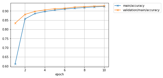
If you continue learning a little more, there is still an atmosphere where you can improve the accuracy a little.

Next, let's use Graphviz to visualize the calculation graph output by ʻExtension called dump_graph`.

%%bash
dot -Tpng mnist_result/cg.dot -o mnist_result/cg.png

\ * Here, I am using Cell magic that uses the bash command on Jupyter notebook. The command on the second line itself is a normal shell command.

Image(filename='mnist_result/cg.png')

Output result

From top to bottom, you can see what Function the data and parameters were passed to for the calculation and the Variable for the loss was output.

8. Infer with a trained model

import numpy as np
from chainer import serializers
from chainer.cuda import to_gpu
from chainer.cuda import to_cpu

model = MLP()
serializers.load_npz('mnist_result/model_epoch-10', model)
model.to_gpu(gpu_id)

%matplotlib inline
import matplotlib.pyplot as plt

x, t = test[0]
plt.imshow(x.reshape(28, 28), cmap='gray')
plt.show()
print('label:', t)

x = to_gpu(x[None, ...])
y = model(x)
y = to_cpu(y.data)

print('predicted_label:', y.argmax(axis=1)[0])

Output result

label: 7
predicted_label: 7

I was able to answer correctly.

Let's write a new network

Here, instead of using the MNIST dataset, try writing various models yourself and experiencing the flow of trial and error using a dataset called CIFAR10, which is a small color image of 32x32 size and labeled with one of the 10 classes. I will.

airplane	automobile	bird	cat	deer	dog	frog	horse	ship	truck

1. Model definition

The model is defined by inheriting the Chain class. Here, let's define a network with a convolution layer instead of the network consisting only of the fully connected layers that we tried earlier. This model has three convolution layers, followed by two fully connected layers.

The definition of the model is mainly done by defining two methods.

1. Define the layers that make up the model with the __init__ constructor --At this time, a layer with optimization target parameters that can be captured from ʻOptimizer by passing a Linkobject that composes the model as a keyword argument usingsuper to the constructor of the parent class (Chain`). Can be added to the model.
2. Write the Forward calculation in the __call__ method called by the()accessor that receives the data.

import chainer
import chainer.functions as F
import chainer.links as L

class MyModel(chainer.Chain):
    
    def __init__(self, n_out):
        super(MyModel, self).__init__(
            conv1=L.Convolution2D(None, 32, 3, 3, 1),
            conv2=L.Convolution2D(32, 64, 3, 3, 1),
            conv3=L.Convolution2D(64, 128, 3, 3, 1),
            fc4=L.Linear(None, 1000),
            fc5=L.Linear(1000, n_out)
        )
        
    def __call__(self, x):
        h = F.relu(self.conv1(x))
        h = F.relu(self.conv2(h))
        h = F.relu(self.conv3(h))
        h = F.relu(self.fc4(h))
        h = self.fc5(h)
        return h

2. Learning

Here, define the train function so that you can easily train another model with the same settings later. this is,

--Model object --Batch size --GPU ID to use --Number of epochs to finish learning --Dataset object

If you pass, it is a function that trains the model internally using the dataset passed using Trainer and returns the model in the state where training is completed.

Let's use this train function to train the MyModel model defined above.

from chainer.datasets import cifar
from chainer import iterators
from chainer import optimizers
from chainer import training
from chainer.training import extensions

def train(model_object, batchsize=64, gpu_id=0, max_epoch=20, train_dataset=None, test_dataset=None):

    # 1. Dataset
    if train_dataset is None and test_dataset is None:
        train, test = cifar.get_cifar10()
    else:
        train, test = train_dataset, test_dataset

    # 2. Iterator
    train_iter = iterators.SerialIterator(train, batchsize)
    test_iter = iterators.SerialIterator(test, batchsize, False, False)

    # 3. Model
    model = L.Classifier(model_object)
    if gpu_id >= 0:
        model.to_gpu(gpu_id)

    # 4. Optimizer
    optimizer = optimizers.Adam()
    optimizer.setup(model)

    # 5. Updater
    updater = training.StandardUpdater(train_iter, optimizer, device=gpu_id)

    # 6. Trainer
    trainer = training.Trainer(updater, (max_epoch, 'epoch'), out='{}_cifar10_result'.format(model_object.__class__.__name__))

    # 7. Evaluator

    class TestModeEvaluator(extensions.Evaluator):

        def evaluate(self):
            model = self.get_target('main')
            model.train = False
            ret = super(TestModeEvaluator, self).evaluate()
            model.train = True
            return ret

    trainer.extend(extensions.LogReport())
    trainer.extend(TestModeEvaluator(test_iter, model, device=gpu_id))
    trainer.extend(extensions.PrintReport(['epoch', 'main/loss', 'main/accuracy', 'validation/main/loss', 'validation/main/accuracy', 'elapsed_time']))
    trainer.extend(extensions.PlotReport(['main/loss', 'validation/main/loss'], x_key='epoch', file_name='loss.png'))
    trainer.extend(extensions.PlotReport(['main/accuracy', 'validation/main/accuracy'], x_key='epoch', file_name='accuracy.png'))
    trainer.run()
    del trainer
    
    return model
    
model = train(MyModel(10), gpu_id=0)  #When running on the CPU`gpu_id=-1`Please specify.

Output result

epoch       main/loss   main/accuracy  validation/main/loss  validation/main/accuracy  elapsed_time
1           1.53309     0.444293       1.29774               0.52707                   5.2449        
2           1.21681     0.56264        1.18395               0.573746                  10.6833       
3           1.06828     0.617358       1.10173               0.609773                  16.0644       
4           0.941792    0.662132       1.0695                0.622611                  21.2535       
5           0.832165    0.703345       1.0665                0.624104                  26.4523       
6           0.729036    0.740257       1.0577                0.64371                   31.6299       
7           0.630143    0.774208       1.07577               0.63953                   36.798        
8           0.520787    0.815541       1.15054               0.639431                  42.1951       
9           0.429535    0.849085       1.23832               0.6459                    47.3631       
10          0.334665    0.882842       1.3528                0.633061                  52.5524       
11          0.266092    0.90549        1.44239               0.635251                  57.7396       
12          0.198057    0.932638       1.6249                0.6249                    62.9918       
13          0.161151    0.944613       1.76964               0.637241                  68.2177       
14          0.138705    0.952145       1.98031               0.619725                  73.4226       
15          0.122419    0.957807       2.03002               0.623806                  78.6411       
16          0.109989    0.962148       2.08948               0.62281                   84.3362       
17          0.105851    0.963675       2.31344               0.617237                  89.5656       
18          0.0984753   0.966289       2.39499               0.624801                  95.1304       
19          0.0836834   0.970971       2.38215               0.626791                  100.36        
20          0.0913404   0.96925        2.46774               0.61873                   105.684       

Learning is over up to 20 epochs. Let's take a look at the loss and accuracy plot.

Image(filename='MyModel_cifar10_result/loss.png')

Image(filename='MyModel_cifar10_result/accuracy.png')

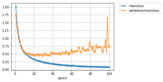
The accuracy (main / accuracy) in the training data has reached around 97%, but the loss (validation / main / loss) in the test data has rather increased with each iteration. Also, the accuracy of the test data (`validation / main / accuracy') has peaked at around 62%. The training data has good accuracy, but the test data does not, so it seems that the ** model is overfitting to the training data **.

3. Prediction using a trained model

The test accuracy was around 62%, but let's try using this trained model to classify some test images.

%matplotlib inline
import matplotlib.pyplot as plt

cls_names = ['airplane', 'automobile', 'bird', 'cat', 'deer',
             'dog', 'frog', 'horse', 'ship', 'truck']

def predict(model, image_id):
    _, test = cifar.get_cifar10()
    x, t = test[image_id]
    model.to_cpu()
    y = model.predictor(x[None, ...]).data.argmax(axis=1)[0]
    print('predicted_label:', cls_names[y])
    print('answer:', cls_names[t])

    plt.imshow(x.transpose(1, 2, 0))
    plt.show()

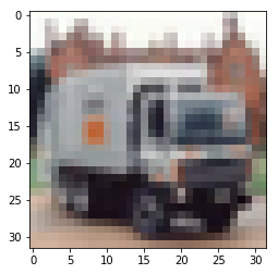
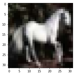
for i in range(10, 15):
    predict(model, i)

Output result

predicted_label: dog
answer: airplane

predicted_label: truck
answer: truck

predicted_label: bird
answer: dog

predicted_label: horse
answer: horse

predicted_label: truck
answer: truck

Some were well classified, others were not. Even if you can get the correct answer in almost 100 shots on the dataset used to train the model, it is meaningless unless you can make highly accurate predictions for unknown data, that is, the images in the test dataset [^ NN]. The accuracy of the test data is said to be related to the ** generalization performance ** of the model.

How can you design and train a model with high generalization performance?

4. Let's define a deeper model

Now let's define a model with more layers than the model above. Here, we define a one-layer convolutional network as ConvBlock and a one-layer fully connected network as LinearBlock, and define a large network by stacking many of them sequentially.

Define components

First, let's define ConvBlock and LinearBlock, which are the components of the large network we are aiming for.

class ConvBlock(chainer.Chain):
    
    def __init__(self, n_ch, pool_drop=False):
        w = chainer.initializers.HeNormal()
        super(ConvBlock, self).__init__(
            conv=L.Convolution2D(None, n_ch, 3, 1, 1,
                                 nobias=True, initialW=w),
            bn=L.BatchNormalization(n_ch)
        )
        
        self.train = True
        self.pool_drop = pool_drop
        
    def __call__(self, x):
        h = F.relu(self.bn(self.conv(x)))
        if self.pool_drop:
            h = F.max_pooling_2d(h, 2, 2)
            h = F.dropout(h, ratio=0.25, train=self.train)
        return h
    
class LinearBlock(chainer.Chain):
    
    def __init__(self):
        w = chainer.initializers.HeNormal()
        super(LinearBlock, self).__init__(
            fc=L.Linear(None, 1024, initialW=w))
        self.train = True
        
    def __call__(self, x):
        return F.dropout(F.relu(self.fc(x)), ratio=0.5, train=self.train)

ConvBlock is defined as a model that inherits Chain. It has one convolution layer and a Batch Normalization layer with parameters, so we are registering these in the constructor. In the __call__ method, while passing data to these, the activation function ReLU is applied, and when pool_drop is passed to the constructor with True, the functions Max Pooling and Dropout are applied. It's a small network.

In Chainer, the forward calculation code itself written using Python represents the structure of the model. In other words, what layer the data went through at run time defines the network itself. This makes it easy to write networks that include branches as described above, and enables flexible, simple, and highly readable network definitions. This is a feature called ** Define-by-Run **.

Definition of a large network

Next, let's stack these small networks as components to define a large network.

class DeepCNN(chainer.ChainList):

    def __init__(self, n_output):
        super(DeepCNN, self).__init__(
            ConvBlock(64),
            ConvBlock(64, True),
            ConvBlock(128),
            ConvBlock(128, True),
            ConvBlock(256),
            ConvBlock(256),
            ConvBlock(256),
            ConvBlock(256, True),
            LinearBlock(),
            LinearBlock(),
            L.Linear(None, n_output)
        )
        self._train = True
            
    @property
    def train(self):
        return self._train
            
    @train.setter
    def train(self, val):
        self._train = val
        for c in self.children():
            c.train = val
    
    def __call__(self, x):
        for f in self.children():
            x = f(x)
        return x

The class we are using here is ChainList. This class inherits from Chain and is useful when defining a network that calls several Links and Chain in sequence. Models defined by inheriting ChainList can pass ** Link or Chain objects as regular arguments instead of ** keyword arguments when calling the constructor of the parent class. And these can be retrieved ** in the order they were registered ** by the ** self.children () ** method.

This feature makes it easy to write forward calculations. From the list of components returned by ** self.children () **, the components are extracted in order by the for statement, and the partial network calculation extracted is applied to the original input x. If you replace x with this output in order, you can apply a series of Links or Chain in the same order as they were registered in the parent class in the constructor. Therefore, it is useful for defining large networks represented by the application of sequential partial networks.

Now let's turn learning. Since there are many parameters this time, set the number of epochs to stop learning to 100.

model = train(DeepCNN(10), max_epoch=100)

Output result

epoch       main/loss   main/accuracy  validation/main/loss  validation/main/accuracy  elapsed_time
1           2.05147     0.242887       1.71868               0.340764                  14.8099       
2           1.5242      0.423816       1.398                 0.48537                   29.12         
3           1.24906     0.549096       1.12884               0.6042                    43.4423       
4           0.998223    0.652649       0.937086              0.688495                  58.291        
5           0.833486    0.720009       0.796678              0.73756                   73.4144       
.
.
.
95          0.0454193   0.987616       0.815549              0.863555                  1411.86       
96          0.0376641   0.990057       0.878458              0.873109                  1426.85       
97          0.0403836   0.98953        0.849209              0.86465                   1441.19       
98          0.0369386   0.989677       0.919462              0.873905                  1456.04       
99          0.0361681   0.990677       0.88796               0.86873                   1470.46       
100         0.0383634   0.988676       0.92344               0.869128                  1484.91     

(Since the log is long, the middle is omitted.)

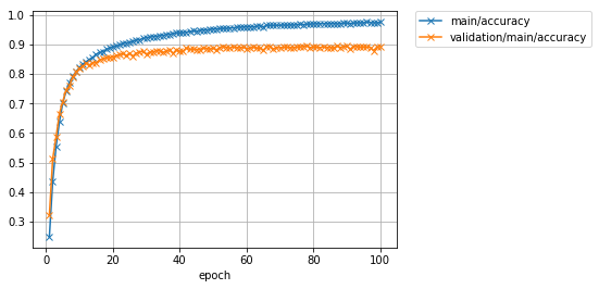
Learning is finished. Let's take a look at the loss and accuracy graph.

Image(filename='DeepCNN_cifar10_result/loss.png')

Image(filename='DeepCNN_cifar10_result/accuracy.png')

You can see that the accuracy of the test data has improved significantly compared to the previous time. The accuracy, which was around 62%, has increased to around 87%. However, the latest research results have achieved nearly 97%. In order to further improve the accuracy, not only the improvement of the model as done this time, but also the operation of artificially increasing the training data (Data augmentation) and the operation of integrating the outputs of multiple models into one output (Ensemble). And so on, various ideas can be considered.

Let's write a dataset class

Here, I will write the dataset class by myself using the function to acquire the data of CIFAR10 already prepared in Chainer. Chainer requires that the class that represents the dataset has the following functionality:

--__len__ method that returns the number of data in the dataset --The get_example method that returns the data or data / label pair that corresponds to the ʻi` passed as an argument.

The functionality required for other datasets can be provided by inheriting the chainer.dataset.DatasetMixin class. Here, let's create a dataset class with the Data augmentation function by inheriting the DatasetMixin class.

1. Write a CIFAR10 dataset class

import numpy as np
from chainer import dataset
from chainer.datasets import cifar

class CIFAR10Augmented(dataset.DatasetMixin):

    def __init__(self, train=True):
        train_data, test_data = cifar.get_cifar10()
        if train:
            self.data = train_data
        else:
            self.data = test_data
        self.train = train
        self.random_crop = 4

    def __len__(self):
        return len(self.data)

    def get_example(self, i):
        x, t = self.data[i]
        if self.train:
            x = x.transpose(1, 2, 0)
            h, w, _ = x.shape
            x_offset = np.random.randint(self.random_crop)
            y_offset = np.random.randint(self.random_crop)
            x = x[y_offset:y_offset + h - self.random_crop,
                  x_offset:x_offset + w - self.random_crop]
            if np.random.rand() > 0.5:
                x = np.fliplr(x)
            x = x.transpose(2, 0, 1)
        return x, t

This class is for each of the CIFAR10 data

--Crop 28x28 area randomly from 32x32 size --Invert left and right with a probability of 1/2

We are doing the processing. It is known that increasing the variation of training data in a pseudo manner by adding such operations is useful for suppressing overfitting. In addition to these operations, methods have been proposed to increase the number of training data in a pseudo manner by various processing such as transformation that changes the color of the image, random rotation, and affine transformation.

If you want to write the data acquisition part yourself, pass the path of the image folder and the path to the text file with the label corresponding to the file name to the constructor and keep it as a property, and in the get_example method You can see that you can read each image and return it with the corresponding label.

2. Learn using the created dataset class

Now let's start learning using this CIFAR10 class. Let's find out how effective Data augmentation is by using the same large network we used earlier. Except for the dataset class, including the train function, it is almost the same as the code used earlier. The only difference is the number of epochs and the name of the destination directory.

model = train(DeepCNN(10), max_epoch=100, train_dataset=CIFAR10Augmented(), test_dataset=CIFAR10Augmented(False))

Output result

epoch       main/loss   main/accuracy  validation/main/loss  validation/main/accuracy  elapsed_time
1           2.023       0.248981       1.75221               0.322353                  18.4387       
2           1.51639     0.43716        1.36708               0.512639                  36.482        
3           1.25354     0.554177       1.17713               0.586087                  54.6892       
4           1.05922     0.637804       0.971438              0.665904                  72.9602       
5           0.895339    0.701886       0.918005              0.706409                  91.4061       
.
.
.  
95          0.0877855   0.973171       0.726305              0.89162                   1757.87       
96          0.0780378   0.976012       0.943201              0.890725                  1776.41       
97          0.086231    0.973765       0.57783               0.890227                  1794.99       
98          0.0869593   0.973512       1.65576               0.878981                  1813.52       
99          0.0870466   0.972931       0.718033              0.891421                  1831.99       
100         0.079011    0.975332       0.754114              0.892815                  1850.46     

(Since the log is long, the middle is omitted.)

It was found that the accuracy, which had peaked at about 87% without Data augmentation, can be improved to 89% or more by applying augmentation to the training data. It's an improvement of just over 2%.

Finally, let's look at the loss and accuracy graph.

Image(filename='DeepCNN_cifar10augmented_result/loss.png')

Output result

Image(filename='DeepCNN_cifar10augmented_result/accuracy.png')

in conclusion

In this article, about Chainer

--How to write a learning loop without using Trainer --How to use Trainer --How to write your own model --How to write your own dataset class

Was briefly introduced. I don't know if it will be done in Hands-on format in the future, but I would like to write an explanation of something like the following somewhere.

--How to make your own Updater and Iterator that make up the Trainer- --How to fine-tun the VGG16Layers and ResNet50Layers Pre-trained models under the chainer.links.models.vision module for specific tasks. --How to make Extension

We also welcome anyone who is committed to the development of Chainer! Since Chainer is open source software, it will evolve by proposing the functions you want and sending pull requests. If you are interested, please read this Contoribution Guide and then make an issue or send a PR. please look. We'll be expecting you.

pfent/chainer https://github.com/pfnet/chainer

footnote

[^ Training and Validation data]: This article focuses on explaining how to use Chainer, so it doesn't make a clear distinction between the Validation and Test datasets. But in reality these should be distinguished. Normally, you would remove some of the Training data from the Training dataset and configure the Validation dataset with the removed data. After that, the general procedure is to evaluate the model trained with the training data first with the validation data, and then improve the model to improve the performance with the validation data. Test data is only used to evaluate the performance of the final model (for example, for comparison with other models) after all efforts have been completed. In some cases, multiple training / validation data configurations may be prepared for the purpose of avoiding overfitting due to model improvement using biased data. [^ NN]: The prediction accuracy for the training data is that data if it can be found by querying some data extracted from the training data and searching from the training dataset that contains it. By answering the label attached, it will be 100%.