[PYTHON] Learn the flow of Bayesian estimation and how to use Pystan through a simple regression model
Introduction
[Introduction to data analysis by Bayesian statistical modeling starting with R and Stan](https://www.amazon.co.jp/%E5%AE%9F%E8%B7%B5Data-Science%E3%82%B7%E3%83] % AA% E3% 83% BC% E3% 82% BA-R% E3% 81% A8Stan% E3% 81% A7% E3% 81% AF% E3% 81% 98% E3% 82% 81% E3% 82 % 8B-% E3% 83% 99% E3% 82% A4% E3% 82% BA% E7% B5% B1% E8% A8% 88% E3% 83% A2% E3% 83% 87% E3% 83% AA% E3% 83% B3% E3% 82% B0% E3% 81% AB% E3% 82% 88% E3% 82% 8B% E3% 83% 87% E3% 83% BC% E3% 82% BF% E5% 88% 86% E6% 9E% 90% E5% 85% A5% E9% 96% 80-KS% E6% 83% 85% E5% A0% B1% E7% A7% 91% E5% AD% A6% I read E5% B0% 82% E9% 96% 80% E6% 9B% B8 / dp / 4065165369). It was easy to understand and I was able to read it without clogging. it's recommended. In order to deepen my understanding, I would like to trace the contents of the book and try it. This book uses R and stan, but here we use Python and Pystan. The general content of this post is as follows:
- Bayes' theorem
- MCMC method
- How to use Pystan
- Simple regression model
You will learn the flow of Bayesian estimation and how to use Pystan through a simple model called a simple regression model.
0. Module
Here, import the required modules in advance.
import numpy as np
import matplotlib.pyplot as plt
import pystan
import arviz

plt.rcParams["font.family"] = "Times New Roman"      #Set the entire font
plt.rcParams["xtick.direction"] = "in"               #Inward the x-axis scale line
plt.rcParams["ytick.direction"] = "in"               #Inward the y-axis scale line
plt.rcParams["xtick.minor.visible"] = True           #Addition of x-axis auxiliary scale
plt.rcParams["ytick.minor.visible"] = True           #Addition of y-axis auxiliary scale
plt.rcParams["xtick.major.width"] = 1.5              #Line width of x-axis main scale line
plt.rcParams["ytick.major.width"] = 1.5              #Line width of y-axis main scale line
plt.rcParams["xtick.minor.width"] = 1.0              #Line width of x-axis auxiliary scale line
plt.rcParams["ytick.minor.width"] = 1.0              #Line width of y-axis auxiliary scale line
plt.rcParams["xtick.major.size"] = 10                #x-axis main scale line length
plt.rcParams["ytick.major.size"] = 10                #Length of y-axis main scale line
plt.rcParams["xtick.minor.size"] = 5                 #x-axis auxiliary scale line length
plt.rcParams["ytick.minor.size"] = 5                 #Length of y-axis auxiliary scale line
plt.rcParams["font.size"] = 14                       #Font size
plt.rcParams["axes.linewidth"] = 1.5                 #Enclosure thickness
1. Bayes' theorem
Bayesian inference is based on Bayes' theorem.
p(\theta|x)=p(\theta) \frac{p(x|\theta)}{\int p(x|\theta)p(\theta)d\theta}
here
(Ex-post distribution) = (Prior distribution) \times \frac{(Likelihood)}{(周辺Likelihood)}
Peripheral likelihood is a normalization constant that sets the integral value of the posterior distribution to 1. Therefore, the following relationship is established by omitting the term of peripheral likelihood.
(Ex-post distribution) \propto (Prior distribution) \times (Likelihood)
1.1 Example
Consider Bayesian estimation of the mean, using a random variable $ x $ that follows a normal distribution as an example. Suppose you know that the standard deviation is 1. The probability density function of the normal distribution is as follows.
\begin{align} p(x|\mu, \sigma=1) &= \frac{1}{\sqrt{2\pi\sigma^2}}\exp{\left(-\frac{(x-\mu)^2}{2\sigma^2}\right)} \\
&= \frac{1}{\sqrt{2\pi}}\exp{\left(-\frac{(x-\mu)^2}{2}\right)} \end{align}
np.random.seed(seed=1) #Random seed

mu = 5.0 #average
s = 1.0 #standard deviation
N = 10 #Quantity
x = np.random.normal(mu,s,N)
print(x)
array([6.62434536, 4.38824359, 4.47182825, 3.92703138, 5.86540763,
       2.6984613 , 6.74481176, 4.2387931 , 5.3190391 , 4.75062962])
Find the probability (likelihood) of obtaining the above data. The data is $ D $. Since the events that obtain each data are independent, the probabilities of obtaining each data are multiplied.
f(D|\mu) = \prod_{i=0}^{N-1} \frac{1}{\sqrt{2\pi}}\exp{\left(-\frac{(x_i-\mu)^2}{2}\right)}
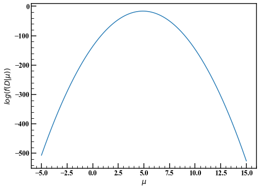
Although not in the book, let's visualize the above function. It seems that the maximum likelihood method is to take the maximum value of the likelihood function and determine that the average is 5 (point estimation).
mu_ = np.linspace(-5.0,15.0,1000)
f_D = 1.0
for x_ in x:
    f_D *= 1.0/np.sqrt(2.0*np.pi) * np.exp(-(x_-mu_)**2 / 2.0) #Likelihood function

fig,axes = plt.subplots(figsize=(8,6))
axes.plot(mu_,np.log(f_D))
axes.set_xlabel(r"$\mu$")
axes.set_ylabel(r"$log (f(D|\mu))$")
Going back to Bayesian inference, we determine the prior distribution. If you don't know the parameter $ \ mu $ in advance, follow the principle of inadequate grounds and consider a wide distribution for the time being. This time, we will use a normal distribution with a variance of 10000 and an average of 0.
In Bayesian inference, the posterior distribution can be complex and difficult to integrate. Even if you obtain the probability density function of the posterior distribution, if you cannot integrate it, for example, the probability that the mean value is between 4 and 6 cannot be obtained. The MCMC method is useful in such cases. In this example, there is only one parameter, so let's divide it by $ \ mu $ instead of the MCMC method and see how the posterior distribution looks.
f_mu = 1.0/np.sqrt(20000.0*np.pi) * np.exp(-mu_**2.0 / 20000) #Prior distribution
f_mu_poster = f_mu * f_D #(Prior distribution)×(Likelihood)
f_mu_poster /= np.sum(f_mu_poster) #Set the integral value to 1

fig,axes = plt.subplots(figsize=(8,6))
axes.plot(mu_,f_mu,label="Prior distribution")
axes.plot(mu_,f_mu_poster,label="Posterior distribution")
axes.legend(loc="best")
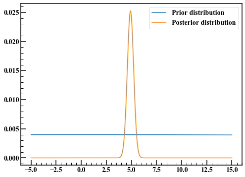
The prior distribution had a wide tail, but the Bayesian updated posterior distribution has a narrow tail. The expected value of the posterior distribution appears to be at 5, as obtained by the maximum likelihood method.
2. MCMC method
The MCMC method is an abbreviation for Markov chain Monte Carlo method. This is a random number generation method that uses Markov chains in which the value at a certain point in time is affected only by the previous point in time. In Bayesian inference, random numbers that follow the posterior distribution of parameters are generated by the MCMC method and used instead of integration. For example, if you want to find the expected value of the posterior distribution, you can find it by calculating the average of the random numbers.
2.1 Metropolis-Hastings method (MH method)
Describes an algorithm that generates random numbers that follow a certain probability distribution. For simplicity, we will only estimate one parameter.
- Determine the initial value of random numbers $ \ hat {\ theta} $.
- Generate random numbers that follow a normal distribution with mean 0 and variance $ \ sigma ^ 2 $.
- Calculate the sum of its random number and the initial value $ \ hat {\ theta} $. Let this be $ \ theta ^ {suggest} $.
- Calculate the ratio of the probability densities of $ \ hat {\ theta} $ and $ \ theta ^ {suggest} $.
- If the ratio of probability densities is greater than 1, then $ \ theta ^ {suggest} $ is adopted, and if it is 1 or less, that value is used as the probability and adopted or rejected.
The adopted random number is used as the initial value and repeated many times. The higher the probability density, the easier it is for random numbers to be adopted, so it feels like it follows the probability distribution. Using the example of 1.1 again, let's generate a random number that follows the posterior distribution by the above method.
np.random.seed(seed=1) #Random seed

def posterior_dist(mu): #Ex-post distribution
    #(Prior distribution)×(Likelihood)
    return 1.0/np.sqrt(20000.0*np.pi) * np.exp(-mu**2.0 / 20000) \
* np.prod(1.0/np.sqrt(2.0*np.pi) * np.exp(-(x-mu)**2 / 2.0))

def MH_method(N,s):
    rand_list = [] #Random numbers adopted
    theta = 1.0 #1.Determine the initial value appropriately

    for i in range(N):
        rand = np.random.normal(0.0,s) #2.Generate random numbers that follow a normal distribution with mean 0 and standard deviation s

        suggest = theta + rand #3.
        dens_rate = posterior_dist(suggest) / posterior_dist(theta) #4.Probability density ratio

        # 5.
        if dens_rate >= 1.0 or np.random.rand() < dens_rate:
            theta = suggest
            rand_list.append(theta)

    return rand_list
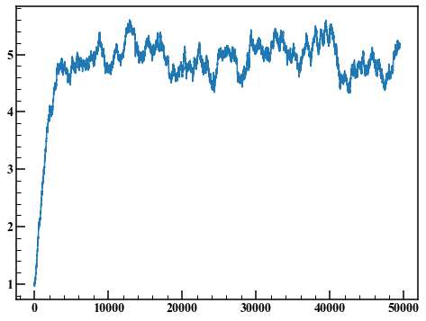
Repeat steps 1 to 5 50,000 times, with the standard deviation of the random numbers generated in step 2 as 1.
rand_list = MH_method(50000,1.0)
len(rand_list) / 50000
0.3619
The probability that a random number will be adopted is called the acceptance rate. This time it was 36.2%.
fig,axes = plt.subplots(figsize=(8,6))
axes.plot(rand_list)
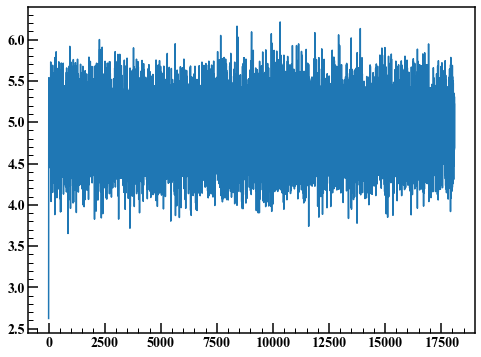
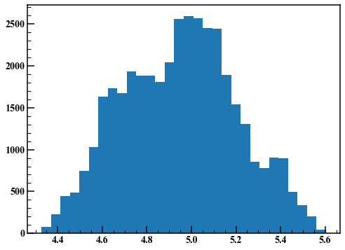
Such a graph is called a trace plot. The first few points are unsteady due to the influence of the initial values. Here, the first 1000 points are discarded and a histogram is drawn.
fig,axes = plt.subplots(figsize=(8,6))
axes.hist(rand_list[1000:],30)
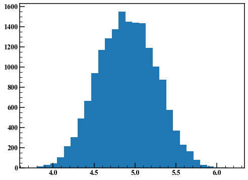
I got a good result. Next, set the standard deviation of the random numbers generated in step 2 to 0.01 and repeat the same procedure.
rand_list = MH_method(50000,0.01)
len(rand_list) / 50000
0.98898
The acceptance rate has increased to 98.9%.
fig,axes = plt.subplots(figsize=(8,6))
axes.plot(rand_list)
Discard the first 10000 points and draw the histogram.
fig,axes = plt.subplots(figsize=(8,6))
axes.hist(rand_list[10000:],30)
As you can see, the result of the MH method depends on the variance of the random numbers used in step 2. The Hamiltonian Monte Carlo method is an algorithm that solves this problem. Stan benefits from a variety of clever algorithms implemented.
3. How to use Pystan
The Stan code requires a data block, a parameters block, and a model block. The data block describes the data information to be used, the parameters block describes the parameters to be estimated, and the model block describes the prior distribution and likelihood. The generated quantities block can generate random numbers using the estimated parameters. I wrote the description method in the comment in the Stan code.
stan_code = """
data {
  int N;          //sample size
  vector[N] x;   //data
}

parameters {
  real mu;       //average
  real<lower=0> sigma;    //standard deviation<lower=0>Specifies that only takes values greater than or equal to 0
}

model {
  //Normal distribution of mean mu, standard deviation sigma
  x ~ normal(mu, sigma); // "~"The symbol indicates that the left side follows the distribution of the right side
}

generated quantities{
  //Get posterior predictive distribution
  vector[N] pred;
  //Unlike Python, subscripts start at 1
  for (i in 1:N) {
    pred[i] = normal_rng(mu, sigma);
  }
}
"""
Compile the Stan code.
sm = pystan.StanModel(model_code=stan_code) #Compile stan code
Summarize the data to be used. Correspond to the variable name declared in the data block of the above Stan code.
#Put together the data
stan_data = {"N":len(x), "x":x}
Before running MCMC, let's take a look at the arguments of the sampling method.
- Number of iterations iter: The number of random numbers generated. If nothing is specified, it defaults to 2000. If the convergence is poor, it may be a large value.
- Burn-in period warmup: Like the trace plot in 2.1, it is initially affected by the initial value. To avoid that effect, discard the points specified by warmup.
- Thinning thin: Adopt one random number for every thin. Since the MCMC method uses Markov chains, it is affected one time ago and has autocorrelation. Reduce this effect.
- Chain chains: In order to evaluate convergence, random numbers are generated by MCMC chains times by changing the initial value. If the results of each trial are similar, it can be determined that they have converged.
Execute MCMC.
#Run MCMC
mcmc_normal = sm.sampling(
    data = stan_data,
    iter = 2000,
    warmup = 1000,
    chains = 4,
    thin = 1,
    seed = 1
)
Display the result. The data used were random numbers that follow a normal distribution with a mean of 5 and a standard deviation of 1. mu is the mean and sigma is the standard deviation. Describes each item in the results table.
- mean: Expected value of posterior distribution
- se_mean: Expected value of posterior distribution divided by the square root of the number of valid samples [^ 1]
- sd: Standard deviation of posterior distribution
- 2.5% -97.5%: Bayesian confidence interval. Arrange the random numbers that follow the posterior distribution in ascending order, and check the values corresponding to the 2.5% to 97.5% points. If you take this difference, you will get a 95% Bayesian confidence interval (confidence interval).
- n_eff: Number of random numbers adopted
- Rhat: Represents the ratio of the variance of all random numbers in the same chain to the average variance of random numbers in the same chain. When chains is 3 or more, Rhat seems to be smaller than 1.1 as a guide.
- lp__: Logarithmic posterior probability [^ 2]
mcmc_normal
Inference for Stan model: anon_model_710b192b75c183bf7f98ae89c1ad472d.
4 chains, each with iter=2000; warmup=1000; thin=1;
post-warmup draws per chain=1000, total post-warmup draws=4000.

           mean se_mean     sd   2.5%    25%    50%    75%  97.5%  n_eff   Rhat
mu          4.9    0.01   0.47    4.0   4.61   4.89   5.18   5.87   1542    1.0
sigma      1.46    0.01   0.43   0.89   1.17   1.38   1.66   2.58   1564    1.0
pred[1]    4.85    0.03   1.58   1.77   3.88   4.86   5.83    8.0   3618    1.0
pred[2]     4.9    0.03   1.62   1.66   3.93    4.9   5.89   8.11   3673    1.0
pred[3]    4.87    0.03    1.6   1.69   3.86   4.85   5.86   8.14   3388    1.0
pred[4]    4.86    0.03   1.57   1.69   3.89   4.87   5.81   7.97   3790    1.0
pred[5]    4.88    0.03    1.6   1.67   3.89   4.89   5.89   7.98   3569    1.0
pred[6]    4.86    0.03   1.61   1.56   3.94   4.87   5.81   8.01   3805    1.0
pred[7]    4.89    0.03    1.6    1.7    3.9   4.88   5.86   8.09   3802    1.0
pred[8]    4.88    0.03   1.61   1.62   3.87   4.88    5.9   8.12   3210    1.0
pred[9]    4.87    0.03    1.6   1.69   3.86   4.87   5.85    8.1   3845    1.0
pred[10]   4.91    0.03   1.63   1.73   3.91   4.88    5.9    8.3   3438    1.0
lp__      -7.63    0.03   1.08 -10.48  -8.03  -7.29  -6.85  -6.57   1159    1.0

Samples were drawn using NUTS at Wed Jan  1 14:32:42 2020.
For each parameter, n_eff is a crude measure of effective sample size,
and Rhat is the potential scale reduction factor on split chains (at
convergence, Rhat=1).
When I tried fit.plot (), WARNING appeared, so follow it.
WARNING:pystan:Deprecation warning.
PyStan plotting deprecated, use ArviZ library (Python 3.5+).
pip install arviz; arviz.plot_trace(fit))
You can easily check the trace plot and posterior distribution.
arviz.plot_trace(mcmc_normal)
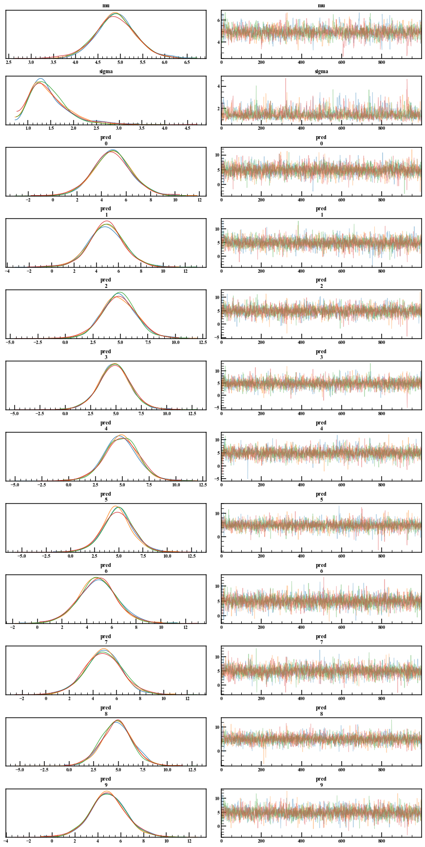
If you want to do something by directly playing with the MCMC sample, or if you want to stick to the graph more, you can extract it with extract. By default, permuted = True, which returns random numbers in mixed order. We want the trace plot to be chronological, so leave this argument False. Also, inc_warmup is whether to include the burn-in period. Also, fit ["variable name"] gave random numbers excluding the burn-in period.
mcmc_extract = mcmc_normal.extract(permuted=False, inc_warmup=True)
mcmc_extract.shape
(2000, 4, 13)
If you check the dimension, it will be (iter, chains, number of parameters). Although the number of graphs is 12, there is a 13th dimension, but when I plot and check it, it looks like lp__.
4. Simple regression analysis
As a summary so far, we will perform a simple regression analysis with Bayesian estimation. Let $ y $ be the response variable and $ x $ be the explanatory variable. Suppose $ y $ follows a normal distribution with mean $ \ mu = ax + b $ and standard deviation $ \ sigma ^ 2 $ with slope $ a $ and intercept $ b $.
\begin{align}
\mu &= ax + b \\
y &\sim \mathcal{N}(\mu,\sigma^2)
\end{align}
It also shows the notations commonly found in other simple regression analysis descriptions.
\begin{align}
y &= ax + b + \varepsilon \\
\varepsilon &\sim \mathcal{N}(0,\sigma^2)
\end{align}
The above two formulas are the same. The first expression shown is more convenient for writing Stan code. In this example, the process of obtaining $ y $ is decided, and the value is sampled from it to perform Bayesian estimation, but in actual data, the process of obtaining data is considered and the result is Bayesian estimation. Look at and make trial and error to modify the model.
4.1 Checking the data
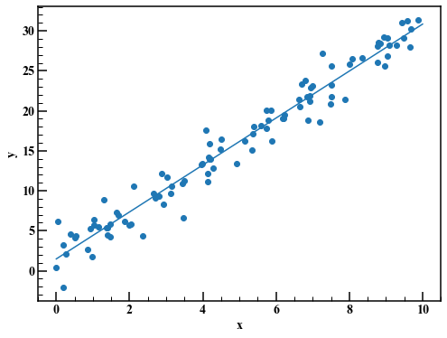
First, create the data you want to use.
np.random.seed(seed=1) #Random seed
a,b = 3.0,1.0 #Slope and intercept
sig = 2.0 #standard deviation
x = 10.0* np.random.rand(100)
y = a*x + b + np.random.normal(0.0,sig,100)
Plot and check. It also displays linear regression using the least squares method.
a_lsm,b_lsm = np.polyfit(x,y,1) #Linear regression with least squares(2.936985017531063, 1.473914508297817)
fig,axes = plt.subplots(figsize=(8,6))
axes.scatter(x,y)
axes.plot(np.linspace(0.0,10.0,100),a_lsm*np.linspace(0.0,10.0,100)+b_lsm)
axes.set_xlabel("x")
axes.set_ylabel("y")
4.2 Consideration of data generation process and creation of Stan code
Assuming that you have completely forgotten the process of creating the data, look at the graph and think that $ y $ and $ x $ are likely to be proportional. Write the Stan code, assuming that the variability follows a normal distribution.
stan_code = """
data {
  int N;          //sample size
  vector[N] x;   //data
  vector[N] y;   //data

  int N_pred; //Predicted sample size
  vector[N_pred] x_pred; //Data to be predicted
}

parameters {
  real a;       //Tilt
  real b;       //Intercept
  real<lower=0> sigma;    //standard deviation<lower=0>Specifies that only takes values greater than or equal to 0
}

transformed parameters {
  vector[N] mu = a*x + b;
}

model {
  // b ~ normal(0, 1000)Specify prior distribution
  //Normal distribution of mean mu, standard deviation sigma
  y ~ normal(mu, sigma); // "~"The symbol indicates that the left side follows the distribution of the right side
}

generated quantities {
  vector[N_pred] y_pred;
  for (i in 1:N_pred) {
    y_pred[i] = normal_rng(a*x_pred[i]+b, sigma);
  }
}
"""
The newly introduced transformed parameters block can create new variables using the variables declared in the parameters block. This time it's a simple formula, so there isn't much difference, but if it's a complicated formula, this will give you a better view. Also, when specifying the prior distribution, write it as "b ~ normal (0, 1000)" in the commented out model block.
4.3 Executing MCMC
Compile the Stan code and run MCMC.
sm = pystan.StanModel(model_code=stan_code) #Compile stan code
x_pred = np.linspace(0.0,11.0,200)
stan_data = {"N":len(x), "x":x, "y":y, "N_pred":200, "x_pred":x_pred}
#Run MCMC
mcmc_linear = sm.sampling(
    data = stan_data,
    iter = 4000,
    warmup = 1000,
    chains = 4,
    thin = 1,
    seed = 1
)
4.4 Checking the results
print(mcmc_linear)
Inference for Stan model: anon_model_28ac7b1919f5bf2d52d395ee71856f88.
4 chains, each with iter=4000; warmup=1000; thin=1;
post-warmup draws per chain=3000, total post-warmup draws=12000.

              mean se_mean     sd   2.5%    25%    50%    75%  97.5%  n_eff   Rhat
a             2.94  9.0e-4   0.06   2.82   2.89   2.94   2.98   3.06   4705    1.0
b             1.47  5.1e-3   0.35   0.79   1.24   1.47   1.71   2.16   4799    1.0
sigma         1.83  1.7e-3   0.13   1.59   1.74   1.82   1.92   2.12   6199    1.0
mu[1]        13.72  1.8e-3   0.19  13.35  13.59  13.72  13.85  14.09  10634    1.0
mu[2]        22.63  2.2e-3   0.24  22.16  22.47  22.63  22.78   23.1  11443    1.0

Samples were drawn using NUTS at Wed Jan  1 15:07:22 2020.
For each parameter, n_eff is a crude measure of effective sample size,
and Rhat is the potential scale reduction factor on split chains (at
convergence, Rhat=1).
It is omitted because it is a very long output. Looking at Rhat, convergence seems to be fine. The 95% confidence interval is illustrated from the posterior prediction distribution.
reg_95 = np.quantile(mcmc_linear["y_pred"],axis=0,q=[0.025,0.975]) #Posterior predictive distribution
fig,axes = plt.subplots(figsize=(8,6))
axes.scatter(x,y,label="Data",c="k")
axes.plot(x_pred,np.average(mcmc_linear["y_pred"],axis=0),label="Expected value")
axes.fill_between(x_pred,reg_95[0],reg_95[1],alpha=0.1,label="95%")
axes.legend(loc="best")
axes.set_xlabel("x")
axes.set_ylabel("y")
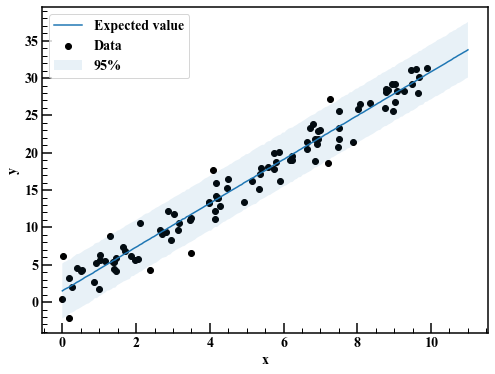
It looks good in general.
Summary
Through Bayesian estimation of a simple regression model, we learned the flow of Bayesian estimation and how to use Stan. Record the flow of Bayesian inference again.
- Check the data: Grasp the structure of the data by plotting it on a graph.
- Consideration of data generation process and creation of Stan code: Write Stan code by formulating the structure of data.
- Run MCMC: Run MCMC to get the posterior distribution.
- Check the result: Check the result and modify the model repeatedly.
This time I used a simple model, but next time I would like to try it with a more general model such as a state space model.
Recommended Posts