Introduction

This is the third installment of PyTorch Official Tutorial following Last time. This time, we will proceed with NEURAL NETWORKS.

Neural Networks

PyTorch builds neural networks using the torch.nn package. Model construction is defined by inheriting nn.Module. nn.Module implements a layer and a forward method that returns output.

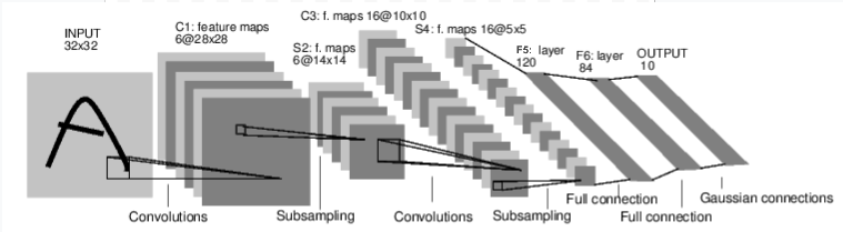
The picture above (flow) is a model that judges the numbers in the image. It takes an input (INPUT 32 x 32), passes through multiple layers, and outputs the result (0 to 9).

The dimensions of each layer change as follows. INPUT（32×32）⇒ C1（6×28×28）⇒ S2（6×14×14）⇒ C3（16×10×10）⇒ S4（6×5×5）⇒ F5（120）⇒ F6（84）⇒ OUTPUT（10）

The learning procedure of the neural network is as follows.

--Define a neural network --Enter the dataset -(Processing of input via network) --Calculate the loss --Reflect the gradient in the network parameters (error backpropagation) --Update network weights

Let's look at each.

Define the network

If you define the network in the picture above, it will be the following code.

import torch
import torch.nn as nn
import torch.nn.functional as F

class Net(nn.Module):

    def __init__(self):
        super(Net, self).__init__()
        # 1 input image channel, 6 output channels, 5x5 square convolution
        # kernel
        self.conv1 = nn.Conv2d(1, 6, 5)
        self.conv2 = nn.Conv2d(6, 16, 5)
        # an affine operation: y = Wx + b
        self.fc1 = nn.Linear(16 * 5 * 5, 120)
        self.fc2 = nn.Linear(120, 84)
        self.fc3 = nn.Linear(84, 10)

    def forward(self, x):
        # Max pooling over a (2, 2) window
        x = F.max_pool2d(F.relu(self.conv1(x)), (2, 2))
        # If the size is a square you can only specify a single number
        x = F.max_pool2d(F.relu(self.conv2(x)), 2)
        x = x.view(-1, self.num_flat_features(x))
        x = F.relu(self.fc1(x))
        x = F.relu(self.fc2(x))
        x = self.fc3(x)
        return x

    def num_flat_features(self, x):
        size = x.size()[1:]  # all dimensions except the batch dimension
        num_features = 1
        for s in size:
            num_features *= s
        return num_features

net = Net()
print(net)

Net(
  (conv1): Conv2d(1, 6, kernel_size=(5, 5), stride=(1, 1))
  (conv2): Conv2d(6, 16, kernel_size=(5, 5), stride=(1, 1))
  (fc1): Linear(in_features=400, out_features=120, bias=True)
  (fc2): Linear(in_features=120, out_features=84, bias=True)
  (fc3): Linear(in_features=84, out_features=10, bias=True)
)

Define each layer with init. torch.nn.Module repeats the calculation starting from the input layer, calculating the coefficients and weights, and passing them to the next layer. This is called forward propagation. torch.nn.Module is a "forward-propagating neural network". Write this forward propagation calculation in the forward method. The above code represents the content of the picture in code. Then, the calculation result of forward propagation can be obtained by the Module.parameters () method.

params = list(net.parameters())
print(len(params))
print(params[0].size())  # conv1's .weight

10
torch.Size([6, 1, 5, 5])

Enter the dataset

[[Autograd: Auto Differentiation](https://pytorch.org/tutorials/beginner/blitz/autograd_tutorial.html#sphx-glr-beginner] in Last time As we saw in -blitz-autograd-tutorial-py), neural networks can also calculate gradients. The gradient is calculated by inputting the input (32x32) suitable for the neural network defined as follows. (Although it is a little different from the sample code, "requires_grad = True" is added so that the gradient can be calculated.)

input = torch.randn(1, 1, 32, 32, requires_grad=True)
out = net(input)
print(out)

tensor([[-0.0769,  0.1520, -0.0556,  0.0384, -0.0847,  0.1081, -0.0190, -0.0522,
         -0.0523, -0.0007]], grad_fn=<AddmmBackward>)

net.zero_grad()
out.backward(torch.randn(1, 10))

Below, you can output the result of back-propagation (back-propagation).

print(input.grad)

Calculate the loss

The Loss Function compares the value output by the network with the teacher data and evaluates how far the training result is from the teacher data. There are several Loss Functions (https://pytorch.org/docs/stable/nn.html#loss-functions) in the nn package. A basic loss function is nn.MSELoss. MSELoss is called the mean squared error, which squares the difference between the training result and the teacher data to find the mean.

output = net(input)
target = torch.randn(10)  # a dummy target, for example
target = target.view(1, -1)  # make it the same shape as output
criterion = nn.MSELoss()

loss = criterion(output, target)
print(loss)

The training result of the neural network is held in output. Set the teacher data in target. (This time it is a random value) Set the loss function to MSELoss. The error between the training result and the teacher data is calculated for loss.

tensor(1.1126, grad_fn=<MseLossBackward>)

Error back propagation

The purpose of learning neural networks is to minimize the error. There are various algorithms (optimization algorithms) for minimizing, but what they have in common is that it is necessary to calculate the gradient. The gradient can be calculated by the backpropagation method. With Pytorch, you can calculate the gradient simply by running loss.backward (). You can see the gradient of conv1 before and after calling loss.backward () in the code below.

net.zero_grad()     #Zero gradient for all parameters (initialization)

print('conv1.bias.grad before backward')
print(net.conv1.bias.grad)

loss.backward()

print('conv1.bias.grad after backward')
print(net.conv1.bias.grad)

conv1.bias.grad before backward
tensor([0., 0., 0., 0., 0., 0.])
conv1.bias.grad after backward
tensor([-0.0033,  0.0033,  0.0027,  0.0030,  0.0031, -0.0053])

Update network weights

As I mentioned earlier, learning adjusts the parameters to minimize the error (loss function). The most basic algorithm (optimization algorithm) for that purpose is the "stochastic gradient descent" (SGD). This tutorial doesn't go into the details of Stochastic Gradient Descent (SGD), but it can be implemented with simple code.

import torch.optim as optim

# create your optimizer
optimizer = optim.SGD(net.parameters(), lr=0.01)

# in your training loop:
optimizer.zero_grad()   # zero the gradient buffers
output = net(input)
loss = criterion(output, target)
loss.backward()
optimizer.step()    # Does the update

In addition to Stochastic Gradient Descent (SGD), there are various optimization algorithms such as Nesterov-SGD, Adam, and RMSProp. The torch.optim package provides various optimization algorithms (optimizers).

Finally

That's it for PyTorch's third tutorial, Neural Networks. I feel that I understand a little about basic neural networks.

Next time would like to proceed with the fourth tutorial "TRAINING A CLASSIFIER".

History

2020/04/22 First edition released 2020/04/29 Next link added

[PYTHON] [PyTorch Tutorial ③] NEURAL NETWORKS