[PYTHON] [PyTorch Tutorial ④] TRAINING A CLASSIFIER
Introduction
This is the 4th installment of PyTorch Official Tutorial following Last time. This time, we will proceed with TRAINING A CLASSIFIER.
Learning class classification
Last time saw how to define a neural network to calculate losses and update network weights. This time, we will use image data to look at the classification problem. PyTorch provides a library torchvision for handling image data. torchvision also comes with basic image datasets such as Imagenet, CIFAR-10, and MNIST. This tutorial uses the CIFAR-10 dataset.
CIFAR-10
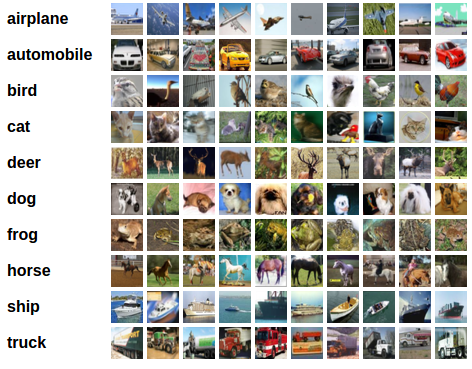
The CIFAR-10 is a 32x32 pixel color image with 3 RGB channels in the shape (3,32,32). Classes are labeled in 10 categories: "Airplane", "Car", "Bird", "Cat", "Deer", "Dog", "Frog", "Horse", "Ship", "Truck" ..
Learning image classification
Let's see the learning flow using CIFAR-10. Learning to classify images involves the following steps in sequence:
- Load and normalize CIFAR10 training and test datasets using torchvision
- Definition of convolutional neural network
- Define the loss function and optimization algorithm
- Learn with training data
- Check the result learned from the test data
1. Loading and normalizing CIFAR-10
It is convenient to use ** Dataset ** and ** DataLoader ** to load data with PyTorch. The Dataset holds the image and the correct label (one training data). DataLoader A utility for repeatedly acquiring training data (test data).
import torch
import torchvision
import torchvision.transforms as transforms

#definition of transform
#Convert to Tensor with ToTensor
#Standardization( X - 0.5) / 0.5
transform = transforms.Compose([
     transforms.ToTensor(),
     transforms.Normalize((0.5, 0.5, 0.5), (0.5, 0.5, 0.5))])

#Training dataset
trainset = torchvision.datasets.CIFAR10(root='./data', train=True,
                                        download=True, transform=transform)

#Training data loader
trainloader = torch.utils.data.DataLoader(trainset, batch_size=4,
                                          shuffle=False, num_workers=2)

#Test dataset
testset = torchvision.datasets.CIFAR10(root='./data', train=False,
                                       download=True, transform=transform)

#Test data loader
testloader = torch.utils.data.DataLoader(testset, batch_size=4,
                                         shuffle=False, num_workers=2)

#List of classifications
classes = ('plane', 'car', 'bird', 'cat',
           'deer', 'dog', 'frog', 'horse', 'ship', 'truck')
First, transform sets the data set transformation method. Compose connects multiple transformations in sequence. Here we are running ToTensor and Normalize. ToTensor converts the image data to Tensor. In ToTensor, RGB values are represented by the fload type [0, 1]. Normalize calculates (X --0.5) / 0.5 and converts the RGB range to [-1, 1].
Some images are displayed with the following code. Since the batch_size of trainloader is 4, 4 images will be processed together.
import matplotlib.pyplot as plt
import numpy as np

#Function to display an image
def imshow(img):
    img = img / 2 + 0.5     #Revert standardization
    npimg = img.numpy()
    plt.imshow(np.transpose(npimg, (1, 2, 0)))


#Get images from training data (random)
dataiter = iter(trainloader)
images, labels = dataiter.next()

#Display image
imshow(torchvision.utils.make_grid(images))
#Show label
print(' '.join('%5s' % classes[labels[j]] for j in range(4)))
frog truck truck deer

2. Definition of convolutional neural network
Copy the neural network from the previous neural network tutorial and modify it to get a 3-channel image (rather than the defined 1-channel image).
import torch.nn as nn
import torch.nn.functional as F


class Net(nn.Module):
    def __init__(self):
        super(Net, self).__init__()
        self.conv1 = nn.Conv2d(3, 6, 5)
        self.pool = nn.MaxPool2d(2, 2)
        self.conv2 = nn.Conv2d(6, 16, 5)
        self.fc1 = nn.Linear(16 * 5 * 5, 120)
        self.fc2 = nn.Linear(120, 84)
        self.fc3 = nn.Linear(84, 10)

    def forward(self, x):
        x = self.pool(F.relu(self.conv1(x)))
        x = self.pool(F.relu(self.conv2(x)))
        x = x.view(-1, 16 * 5 * 5)
        x = F.relu(self.fc1(x))
        x = F.relu(self.fc2(x))
        x = self.fc3(x)
        return x

net = Net()
3. Define the loss function and optimization algorithm
In classification problems, the loss function mainly utilizes the cross entropy error function. For binary classification problems, torch.nn.BCEWithLogitsLoss For multiclass classification problems, torch.nn.CrossEntropyLoss Is often used. Since this time we have 10 label classifications (multi-class classification), we will use CrossEntropyLoss. The optimization algorithm should be the most basic "stochastic gradient descent" (SGD).
import torch.optim as optim

criterion = nn.CrossEntropyLoss()
optimizer = optim.SGD(net.parameters(), lr=0.001, momentum=0.9)
4. Learn with training data
Loop through the data loader and stream training data over the network to optimize parameters.
for epoch in range(2):  #Epoch several loops

    running_loss = 0.0
    for i, data in enumerate(trainloader, 0):
        #Get training data
        inputs, labels = data

        #Initialize the gradient
        optimizer.zero_grad()

        #Pass data through a neural network and calculate forward propagation
        outputs = net(inputs)
        #Error calculation
        loss = criterion(outputs, labels)
        #Backpropagation calculation
        loss.backward()
        #Weight calculation
        optimizer.step()

        #Show status
        running_loss += loss.item()
        if i % 2000 == 1999:    # 2,000 data each
            print('[%d, %5d] loss: %.3f' %
                  (epoch + 1, i + 1, running_loss / 2000))
            running_loss = 0.0

print('Finished Training')
Learning will be completed in about 2 minutes.
[1,  2000] loss: 2.153
[1,  4000] loss: 1.830
[1,  6000] loss: 1.654
[1,  8000] loss: 1.556
[1, 10000] loss: 1.524
[1, 12000] loss: 1.511
[2,  2000] loss: 1.441
[2,  4000] loss: 1.380
[2,  6000] loss: 1.384
[2,  8000] loss: 1.358
[2, 10000] loss: 1.335
[2, 12000] loss: 1.320
Finished Training
5. Check the results learned from the test data
Check the learned result with test data. Let's take a look at some of the test data.
dataiter = iter(testloader)
images, labels = dataiter.next()

# print images
imshow(torchvision.utils.make_grid(images))
print('Teacher data: ', ' '.join('%5s' % classes[labels[j]] for j in range(4)))
Teacher data: cat ship ship plane

Let's see how the model (classifier) that learned these four images judges. Pass the test data to the trained network and you will get the results.
outputs = net(images)
print(outputs[0,:])
tensor([-1.0291, -3.1352,  0.5837,  3.7728, -1.3638,  3.4090,  0.4094,  0.3352,
        -0.6388, -1.4808], grad_fn=<SliceBackward>)
The weight of each label (10) is returned in output.
_, predicted = torch.max(outputs, 1)

print('Predicted: ', ' '.join('%5s' % classes[predicted[j]]
                              for j in range(4)))
Get the maximum index with max. If you specify two return values for max, the index with the maximum value is returned first and the index with the maximum value is returned second.
Predicted: cat ship ship plane
It was confirmed that it matches the teacher data.
Let's check the result with the whole test data.
correct = 0
total = 0
with torch.no_grad():
    for data in testloader:
        images, labels = data
        outputs = net(images)
        _, predicted = torch.max(outputs.data, 1)
        total += labels.size(0)
        correct += (predicted == labels).sum().item()

print('Accuracy of the network on the 10000 test images: %d %%' % (
    100 * correct / total))
Accuracy of the network on the 10000 test images: 52 %
With 10,000 test data, the correct answer rate was 52%. If you haven't learned, it's 1/10 (10%), so you can learn something, but it's not very accurate. Let's look at the correct answer rate for each label.
class_correct = list(0. for i in range(10))
class_total = list(0. for i in range(10))
with torch.no_grad():
    for data in testloader:
        images, labels = data
        outputs = net(images)
        _, predicted = torch.max(outputs, 1)
        c = (predicted == labels).squeeze()
        for i in range(4):
            label = labels[i]
            class_correct[label] += c[i].item()
            class_total[label] += 1


for i in range(10):
    print('Accuracy of %5s : %2d %%' % (
        classes[i], 100 * class_correct[i] / class_total[i]))
Accuracy of plane : 65 %
Accuracy of   car : 51 %
Accuracy of  bird : 33 %
Accuracy of   cat : 22 %
Accuracy of  deer : 39 %
Accuracy of   dog : 64 %
Accuracy of  frog : 66 %
Accuracy of horse : 70 %
Accuracy of  ship : 53 %
Accuracy of truck : 61 %
It seems that there are cases such as cat that I have not learned much.
Learning on GPU
Finally, let's look at learning on the GPU. If you have a GPU-enabled environment, you can use it to train neural networks. If you are using Google Colaboratory, you can use the GPU by selecting "Runtime" ⇒ "Change Runtime Type" ⇒ "GPU".
You can check the GPU usage with the following code.
device = torch.device("cuda:0" if torch.cuda.is_available() else "cpu")
# Assume that we are on a CUDA machine, then this should print a CUDA device:
print(device)
If the device is "cuda", you can use the GPU. If you want to take advantage of the GPU, you need to write code to transfer the model to the GPU.
net.to(device)
Similarly, the training data must be transferred to the GPU.
inputs, labels = inputs.to(device), labels.to(device)
I checked the time taken to study this tutorial on Google Colaboratory Without GPU: 2 minutes 10 seconds When using GPU: 1 minute 40 seconds was. If the dimensions of the training data are not that complex, the effect seems weak.
At the end
That's the content of PyTorch's fourth tutorial, "TRAINING A CLASSIFIER". I was able to understand the basic flow of learning.
Next time, I would like to proceed with the fifth tutorial "LEARNING PYTORCH WITH accurately".
History
2020/04/29 First edition released
Recommended Posts