Python: Diagram of 2D data distribution (kernel density estimation)
Introduction
I wanted to see the distribution state of the data distributed in two dimensions, so I tried to estimate the kernel density with `scipy.stats.gaussian_kde```. The result diagram is as follows. ( bw_method ='scott'`` )

By the way, the simple regression analysis is done smoothly with numpy as follows. (When doing various things, it is important that such code comes out immediately and can be used, so I dare to write it out.)
def sreq(x,y):
    # y=a*x+b
    res=np.polyfit(x, y, 1)
    a=res[0]
    b=res[1]
    coef = np.corrcoef(x, y)
    r=coef[0,1]
    return a,b,r
How to do
The method was as follows. Thank you, poster.
The ingenuity is as follows.
Since the + display is more straightforward on the logarithmic axis, I chose the logarithmic axis, but I also wanted to read the values on the axis, so I drew the logarithmic axis manually. Data processing is performed by taking the common logarithm of raw data.
- I controlled the interval of drawing contour lines by myself. Since the probability density can be obtained with
gaussian_kde, set the top of this value to 1 and draw a line at
Try changing the parameters. .. ..
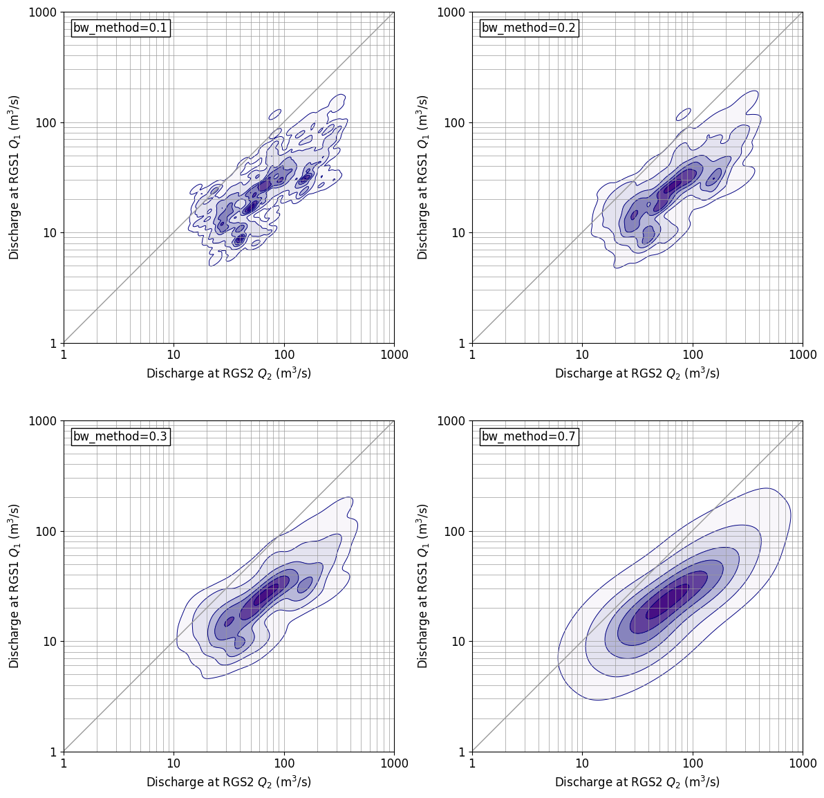
gaussin_bw for kde_There is a parameter called method, and if you change this, you can change the fineness of displaying the distribution shape. The result diagram shown above is the default, bw_method=In the case of ‘scott’, bw below_The figure when the method is changed is shown. bw_method=0.If it is 3, the distribution is close to default. bw_As the value of method increases, the display becomes coarser and bw_method=0.If it is 7, the display is close to the normal two-dimensional normal distribution.
## program
The program that created the result diagram shown in "Introduction" is shown below. If you want to try this program, please try to make the data as you like.
```python
import numpy as np
import pandas as pd
import matplotlib.pyplot as plt
import matplotlib.cm as cm
from scipy.stats import gaussian_kde
def sreq(x,y):
# y=a*x+b
res=np.polyfit(x, y, 1)
a=res[0]
b=res[1]
coef = np.corrcoef(x, y)
r=coef[0,1]
return a,b,r
def inp_obs():
fnameR='df_rgs1_tank_inp.csv'
df1_obs=pd.read_csv(fnameR, header=0, index_col=0) # read excel data
df1_obs.index = pd.to_datetime(df1_obs.index, format='%Y/%m/%d')
df1_obs=df1_obs['2016/01/01':'2018/12/31']
#
fnameR='df_rgs2_tank_inp.csv'
df2_obs=pd.read_csv(fnameR, header=0, index_col=0) # read excel data
df2_obs.index = pd.to_datetime(df2_obs.index, format='%Y/%m/%d')
df2_obs=df2_obs['2016/01/01':'2018/12/31']
#
return df1_obs,df2_obs
def drawfig(x,y,sstr,fnameF):
fsz=12
xmin=0; xmax=3
ymin=0; ymax=3
plt.figure(figsize=(12,6),facecolor='w')
plt.rcParams['font.size']=fsz
plt.rcParams['font.family']='sans-serif'
#
for iii in [1,2]:
nplt=120+iii
plt.subplot(nplt)
plt.xlim([xmin,xmax])
plt.ylim([ymin,ymax])
plt.xlabel('Discharge at RGS2 $Q_2$ (m$^3$/s)')
plt.ylabel('Discharge at RGS1 $Q_1$ (m$^3$/s)')
plt.gca().set_aspect('equal',adjustable='box')
plt.xticks([0,1,2,3], [1,10,100,1000])
plt.yticks([0,1,2,3], [1,10,100,1000])
bb=np.array([1,2,3,4,5,6,7,8,9,10,20,30,40,50,60,70,80,90,100,200,300,400,500,600,700,800,900,1000])
bl=np.log10(bb)
for a0 in bl:
plt.plot([xmin,xmax],[a0,a0],'-',color='#999999',lw=0.5)
plt.plot([a0,a0],[ymin,ymax],'-',color='#999999',lw=0.5)
plt.plot([xmin,xmax],[ymin,ymax],'-',color='#999999',lw=1)
#
if iii==1:
plt.plot(x,y,'o',ms=2,color='#000080',markerfacecolor='#ffffff',markeredgewidth=0.5)
a,b,r=sreq(x,y)
x1=np.min(x)-0.1; y1=a*x1+b
x2=np.max(x)+0.1; y2=a*x2+b
plt.plot([x1,x2],[y1,y2],'-',color='#ff0000',lw=2)
tstr=sstr+'\n$\log(Q_1)=a * \log(Q_2) + b$'
tstr=tstr+'\na={0:.3f}, b={1:.3f} (r={2:.3f})'.format(a,b,r)
#
if iii==2:
tstr=sstr+'\n(kernel density estimation)'
xx,yy = np.mgrid[xmin:xmax:0.01,ymin:ymax:0.01]
positions = np.vstack([xx.ravel(),yy.ravel()])
value = np.vstack([x,y])
kernel = gaussian_kde(value, bw_method='scott')
#kernel = gaussian_kde(value, bw_method=0.1)
f = np.reshape(kernel(positions).T, xx.shape)
f=f/np.max(f)
ll=[0.01, 0.1, 0.3, 0.5, 0.7, 0.9, 1.0]
plt.contourf(xx,yy,f,cmap=cm.Purples,levels=ll)
plt.contour(xx,yy,f,colors='#000080',linewidths=0.7,levels=ll)
xs=xmin+0.03*(xmax-xmin)
ys=ymin+0.97*(ymax-ymin)
plt.text(xs, ys, tstr, ha='left', va='top', rotation=0, size=fsz,
bbox=dict(boxstyle='square,pad=0.2', fc='#ffffff', ec='#000000', lw=1))
#
plt.tight_layout()
plt.savefig(fnameF, dpi=100, bbox_inches="tight", pad_inches=0.1)
plt.show()
def main():
df1_obs, df2_obs =inp_obs()
fnameF='_fig_cor_test1.png'
sstr='Observed discharge (2016-2018)'
xx=df2_obs['Q'].values
yy=df1_obs['Q'].values
xx=np.log10(xx)
yy=np.log10(yy)
drawfig(xx,yy,sstr,fnameF)
#==============
# Execution
#==============
if __name__ == '__main__': main()
that's all
Recommended Posts