Let's build a belief propagation method (Python)

What is belief propagation?

Belief propagation is also called Belief Propagation, and is an algorithm for efficiently finding the marginal distribution of the state of each node on a graphical model such as Bayesian network or Markov random field (MRF). .. Originally, when trying to find this marginal distribution, if the number of nodes is N and the number of states is K, the amount of calculation is $ O (K ^ N) $, and if the number of nodes increases, the calculation cannot be performed in a finite time. However, if this belief propagation method is used, it becomes $ O (NK ^ 2) $ and can be calculated in a finite time. What is convenient when this marginal distribution is obtained is that, depending on the structure of the graph, the optimum state of each node can be obtained using the marginal distribution, or a solution close to it can be obtained even if it is not the optimal solution. This time I tried to build this belief propagation method in Python, so I would like to explain the code step by step.

Program explanation

Usage data

This time, I would like to apply the belief propagation method to the noisy image of Mr. Lena to remove the noise. The values taken by each pixel are two values, 0 and 1.

program

First, add noise to the original image. The code looks like this:

python

def addNoise(image):
    output = np.copy(image)
    flags  = np.random.binomial(n=1, p=0.05, size=image.shape)

    for i in range(image.shape[0]):
        for j in range(image.shape[1]):
            if flags[i,j]:
                output[i,j] = not(output[i,j])

    return output

Next, consider each pixel in the image as a node and build an MRF. Of particular note in this MRF class is the belief Propagation function. Since the Markov random field on the image is a network with a loop structure, it is necessary to repeat message transmission multiple times. This time, it repeats iter times. Initialize the message received by each node from the adjacent node with 1 before repeating the transmission. After entering the send loop, continue sending messages to neighboring nodes with the sendMessage method, and finally integrate the messages from neighboring nodes that you have for each node and calculate the marginal distribution. The marginal method does this.

python

class MRF:
    def __init__(self):
        self.nodes = [] #Node on MRF
        self.id = {} #Node ID
    
    #Add a node to the MRF
    def addNode(self, id, node):
        self.nodes.append(node)
        self.id[id] = node
    
    #Returns the node according to the ID
    def getNode(self, id):
        return self.id[id]
    
    #Returns all nodes
    def getNodes(self):
        return self.nodes
    
    #Start belief propagation
    def beliefPropagation(self, iter=20):
        
        #Initialize messages from neighboring nodes for each node
        for node in self.nodes:
            node.initializeMessage()
        
        #Repeat a certain number of times
        for t in range(iter):
            print(t)
            
            #For each node, send a message to the nodes adjacent to that node
            for node in self.nodes:
                for neighbor in node.getNeighbor():
                    neighbor.message[node] = node.sendMessage(neighbor)
        
        #Calculate the marginal distribution for each node
        for node in self.nodes:
            node.marginal()

Next, define the node class.

python

class Node(object):
    def __init__(self, id):
        self.id = id
        self.neighbor = []
        self.message = {}
        self.prob = None
        
        #Parameters for energy function
        self.alpha = 10.0
        self.beta = 5.0

    def addNeighbor(self, node):
        self.neighbor.append(node)

    def getNeighbor(self):
        return self.neighbor
    
    #Initialize messages from neighboring nodes
    def initializeMessage(self):
        for neighbor in self.neighbor:
            self.message[neighbor] = np.array([1.0, 1.0])
    
    #Integrate all messages
    #prob is marginal distribution
    def marginal(self):
        prob = 1.0

        for message in self.message.values():
            prob *= message

        prob /= np.sum(prob)
        self.prob = prob
    
    #Calculate the likelihood considering the state of the adjacent node
    def sendMessage(self, target):
        neighbor_message = 1.0
        for neighbor in self.message.keys():
            if neighbor != target:
                neighbor_message *= self.message[neighbor]

        compatibility_0 = np.array([np.exp(-self.beta * np.abs(0.0 - 0.0)), np.exp(-self.beta * np.abs(0.0 - 1.0))])
        compatibility_1 = np.array([np.exp(-self.beta * np.abs(1.0 - 0.0)), np.exp(-self.beta * np.abs(1.0 - 1.0))])

        message = np.array([np.sum(neighbor_message * compatibility_0), np.sum(neighbor_message * compatibility_1)])
        message /= np.sum(message)

        return message
    
    #Likelihood calculated from observed values
    def calcLikelihood(self, value):
        likelihood = np.array([0.0, 0.0])

        if value == 0:
            likelihood[0] = np.exp(-self.alpha * 0.0)
            likelihood[1] = np.exp(-self.alpha * 1.0)
        else:
            likelihood[0] = np.exp(-self.alpha * 1.0)
            likelihood[1] = np.exp(-self.alpha * 0.0)

        self.message[self] = likelihood

The important ones are the calcLikelihood, sendMessage, and marginal methods. Suppose you want to send a message from node 1 to node 2 as shown in Figure 1. This message is to tell you what value node 2 should take when you look at node 2 from node 1.

In order to calculate it, it is first necessary to calculate the reliability (validity when the value is taken) for each value of node 1. First, calculate the reliability when looking only at the observed value of node 1. The calcLikelihood method calculates this. If the observed value is 0, the confidence that the node will take 0 increases, and conversely, the confidence that the node will take 1 decreases. If the observed value is 1, the opposite is true.

Next, multiply the reliability calculated from the observed values by the reliability of each value of node 1 when viewed from node 4 (message from node 4 to node 1). Figure 2 shows these. In this calculation, in the code, in the sendMessage method

python

neighbor_message = 1.0
        for neighbor in self.message.keys():
            if neighbor != target:
                neighbor_message *= self.message[neighbor]

This is the

part. </ p>

And use these to calculate the message to send to node 2. The message (reliability) is calculated as follows.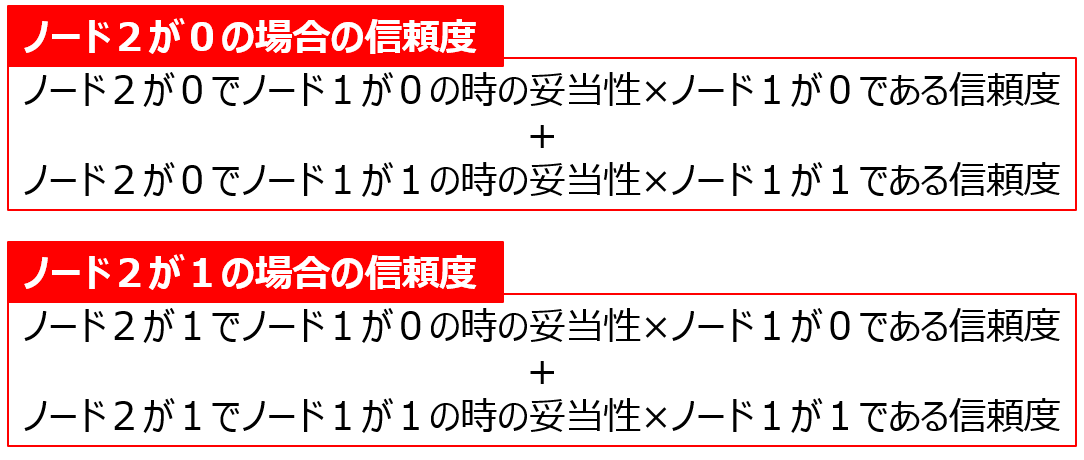 

This is calculated in the sendMessage method

python

compatibility_0 = np.array([np.exp(-self.beta * np.abs(0.0 - 0.0)), np.exp(-self.beta * np.abs(0.0 - 1.0))])
compatibility_1 = np.array([np.exp(-self.beta * np.abs(1.0 - 0.0)), np.exp(-self.beta * np.abs(1.0 - 1.0))])

message = np.array([np.sum(neighbor_message * compatibility_0), np.sum(neighbor_message * compatibility_1)])
message /= np.sum(message)

It will be

. </ P>

Send a message to adjacent nodes on all nodes. After repeating this multiple times, the marginal method is used to multiply all the messages received by the node from the adjacent node to obtain the marginal distribution, and the value that the node should take can be found.

Next, create a function to construct a Markov random field.

python

#Create a node for each pixel and create a connection with an adjacent pixel node
def generateBeliefNetwork(image):
    network = MRF()
    height, width = image.shape

    for i in range(height):
        for j in range(width):
            nodeID = width * i + j
            node = Node(nodeID)
            network.addNode(nodeID, node)

    dy = [-1, 0, 0, 1]
    dx = [0, -1, 1, 0]

    for i in range(height):
        for j in range(width):
            node = network.getNode(width * i + j)

            for k in range(4):
                if i + dy[k] >= 0 and i + dy[k] < height and j + dx[k] >= 0 and j + dx[k] < width:
                    neighbor = network.getNode(width * (i + dy[k]) + j + dx[k])
                    node.addNeighbor(neighbor)

    return network

The last is the main function

python

import numpy as np
import cv2
import matplotlib.pyplot as plt
from skimage.filters import threshold_otsu

def main():
    #Usage data
    image = cv2.imread("Lenna.png ", 0)
    binary = image > threshold_otsu(image).astype(np.int)
    noise = addNoise(binary)
    
    #MRF construction
    network = generateBeliefNetwork(image)
    
    #Create likelihood from observed values (pixel values)
    for i in range(image.shape[0]):
        for j in range(image.shape[1]):
            node = network.getNode(image.shape[1] * i + j)
            node.calcLikelihood(noise[i,j])
    
    #Perform belief propagation
    network.beliefPropagation()
    
    #Marginal distribution[Probability of 0,Probability of 1]Order
    #If the probability of 1 is large, change the pixel value of output to 1.
    output = np.zeros(noise.shape)

    for i in range(output.shape[0]):
        for j in range(output.shape[1]):
            node = network.getNode(output.shape[1] * i + j)
            prob = node.prob
            if prob[1] > prob[0]:
                output[i,j] = 1
    
    #Result display
    plt.gray()
    plt.subplot(121)
    plt.imshow(noise)
    plt.subplot(122)
    plt.imshow(output)
    plt.show()

Execution result

You can see that most of the noise has been removed and the original image has been restored. The formula itself is quite difficult, but it is quite easy to formulate it with a program. This time, we dealt with the discrete case where the number of states is binary, but when dealing with continuous states such as tracking, it is necessary to use the continuous variable version of belief propagation. Various things have been proposed, but next time I would like to build Mean shift Belief Propagation, which is relatively easy to build.

References / Sites

Implementing Markov Random Field / Belief Propagation with Python networkx

Denoising by belief propagation is performed using the famous library for graph theory networkX. It is very easy to understand because it explains the algorithm using figures.

Introduction to Image Processing Technology by Probabilistic Model-Tanaka Laboratory

It seems to be a powerpoint written by a professor in a certain laboratory at Tohoku University. It explains in an easy-to-understand manner using figures and mathematical formulas.