[PYTHON] Take a closer look at the Kaggle / Titanic tutorial
Introduction
I tried Tutorial in Kaggle's Titanic. Random by copy and paste I was able to make predictions using the forest, but before moving on to the next step, I checked what I was doing in the tutorial. You can find many Kaggle Titanic documentation online, but here's a summary of what I thought along with the tutorial.
Check the data
head()
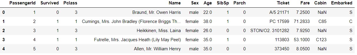
In Tutorial, after reading the data, we use head () to check the data.
train_data.head()
test_data.head()
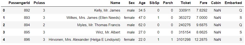
Of course, test_data doesn't have a term for Survived.
describe()
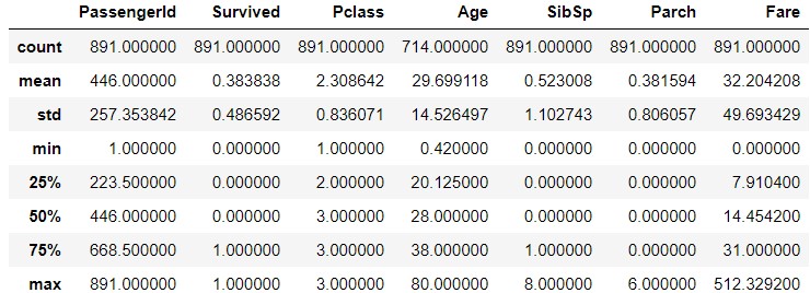
You can see the data statistics with describe (). You can display the object data with describe (include ='O').
train_data.describe()
train_data.describe(inlude='O')
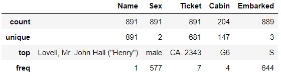
If you look at the Ticket, you'll see that CA.2343 appears seven times. Does this mean that you're a family member or something and you have a ticket with the same number? Similarly, in Cabin, G6 has appeared four times. Does that mean there are four people in the same room? I'm curious if the same family and people in the same room shared their destiny.
test_data.describe()
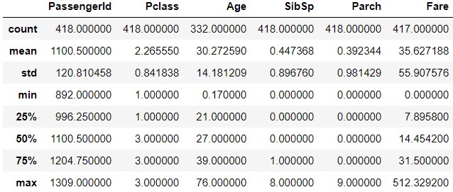
test_data.describe(include='O')
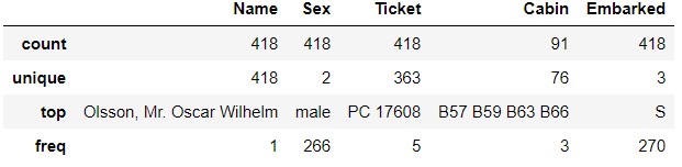 On the
 test_data side, PC 17608 appears 5 times in Ticket. B57 B59 B63 B66 appears 3 times in Cabin.
info()
You can also get data information with info ().
train_data.info()

<class 'pandas.core.frame.DataFrame'>
RangeIndex: 891 entries, 0 to 890
Data columns (total 12 columns):
 #   Column       Non-Null Count  Dtype
---  ------       --------------  -----
 0   PassengerId  891 non-null    int64
 1   Survived     891 non-null    int64
 2   Pclass       891 non-null    int64
 3   Name         891 non-null    object
 4   Sex          891 non-null    object
 5   Age          714 non-null    float64
 6   SibSp        891 non-null    int64
 7   Parch        891 non-null    int64
 8   Ticket       891 non-null    object
 9   Fare         891 non-null    float64
 10  Cabin        204 non-null    object
 11  Embarked     889 non-null    object
dtypes: float64(2), int64(5), object(5)
memory usage: 83.7+ KB
You can see that the number of rows of data is 891, but only 714 for Age, 204 for Cabin, and 889 for Embarked (sorry!).
test_data.info()

<class 'pandas.core.frame.DataFrame'>
RangeIndex: 418 entries, 0 to 417
Data columns (total 11 columns):
 #   Column       Non-Null Count  Dtype
---  ------       --------------  -----
 0   PassengerId  418 non-null    int64
 1   Pclass       418 non-null    int64
 2   Name         418 non-null    object
 3   Sex          418 non-null    object
 4   Age          332 non-null    float64
 5   SibSp        418 non-null    int64
 6   Parch        418 non-null    int64
 7   Ticket       418 non-null    object
 8   Fare         417 non-null    float64
 9   Cabin        91 non-null     object
 10  Embarked     418 non-null    object
dtypes: float64(2), int64(4), object(5)
memory usage: 36.0+ KB
In test_data, the missing data are Age, Fare, Cabin. In train_data, there was missing data in Embarked, but in test_data, they are complete. , Fare was aligned in train_data, but one is missing in test_data.
corr (); See data correlation
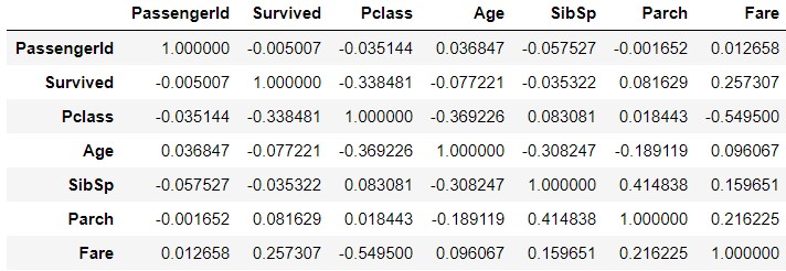
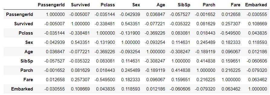
You can check the correlation of each data with `corr ().
train_corr = train_data.corr()
train_corr
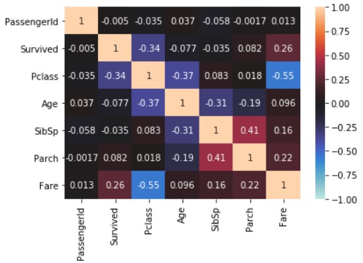
Visualize using seaborn.
import seaborn
import matplotlib.pyplot as plt
seaborn.heatmap(train_data_map_corr, annot=True, vmax=1, vmin=-1, center=0)
plt.show()
The above does not reflect the data of the object type. So, replace the symbols Sex and Embarked with numbers and try the same thing. When copying the data, explicitly copy () Create another data using .
train_data_map = train_data.copy()
train_data_map['Sex'] = train_data_map['Sex'].map({'male' : 0, 'female' : 1})
train_data_map['Embarked'] = train_data_map['Embarked'].map({'S' : 0, 'C' : 1, 'Q' : 2})
train_data_map_corr = train_data_map.corr()
train_data_map_corr
seaborn.heatmap(train_data_map_corr, annot=True, vmax=1, vmin=-1, center=0)
plt.show()
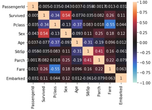
Focus on the Survived line. In the tutorial, we learned with Pclass, Sex, SibSp, and Parch, but Age, Fare, and Embarked are also with Survived. High correlation.
Learning
get_dummies()
from sklearn.ensemble import RandomForestClassifier

y = train_data["Survived"]

features = ["Pclass", "Sex", "SibSp", "Parch"]
X = pd.get_dummies(train_data[features])
X_test = pd.get_dummies(test_data[features])
Learn using scikit-learn. There are four features to use: Pclass, Sex, SibSp, and Parch (features without defects), as defined by features. ..
The data used for training is processed by pd.get_dummies. Pd.get_dummies converts a variable of type object to a dummy variable here.
train_data[features].head()
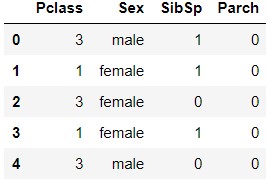
X.head()
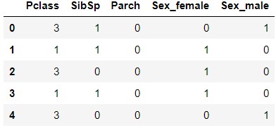
You can see that the feature quantity Sex has changed to Sex_female and Sex_male.
RandomForestClassfier()
Learn using the random forest algorithm RandomForestClassifier ().
model = RandomForestClassifier(n_estimators=100, max_depth=5, random_state=1)
model.fit(X, y)
predictions = model.predict(X_test)
Check the parameters of RandomForestClassifier (the description is about)
| Parameters | Explanation |
|---|---|
| n_estimators | Number of decision trees.The default is 10 |
| max_depth | Maximum depth of decision tree.The default is None(Deepen until completely separated) |
| max_features | For optimal division,How many features to consider.The default isautoso, n_featuresBecome the square root of |
Even though there are only 4 features (5 as dummy variables), making 100 decision trees seems like over-making. This will be verified at a later date.
Check the obtained model
score
print('Train score: {}'.format(model.score(X, y)))

Train score: 0.8159371492704826
The model itself fits 0.8159 (not so expensive).
feature_importances_ Check the importance of features (note the place where the plural s is attached)
x_importance = pd.Series(data=model.feature_importances_, index=X.columns)
x_importance.sort_values(ascending=False).plot.bar()
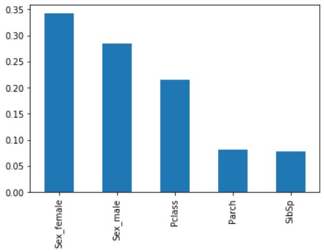
Sex (Sex_female and Sex_male) are of high importance, followed by Pclass. Parch and SibSp are just as low.
Display of decision tree (dtreeviz)
Visualize what kind of decision tree was created. There are various means, but here we will use dtreeviz.
Installation
(Reference; Installation procedure of dtreeviz and grahviz to visualize the result of Python random forest)
Let's assume Windows10 / Anaconda3. First, use pip and conda to install the necessary software.
> pip install dtreeviz
> conda install graphviz
In my case, I got the error "Cannot write" in conda. Restart Anaconda in administrator mode (right-click Anaconda and select" *** Start in administrator mode *** " Select and launch), run conda.
After that, add the folder containing dot.exe to PATH in the system environment.
> dot -V
dot - graphviz version 2.38.0 (20140413.2041)
If you can execute dot.exe as above, it's OK.
Display of decision tree
from dtreeviz.trees import dtreeviz
viz = dtreeviz(model.estimators_[0], X, y, target_name='Survived', feature_names=X.columns, class_names=['Not survived', 'Survived'])
viz

I'm addicted to ***, in the arguments of dtreeviz, the following items.
--model.estimators_ [0]; If you do not specify [0], an error will occur. Since only one of multiple decision trees will be displayed, specify it with [0] etc.
--feature_names; Initially, features was specified, but an error. Actually, since it was made into a dummy variable with pd.dummies () during learning, X.columns after making it a dummy variable To specify
I was a little impressed when I was able to display the decision tree properly.
Finally
By carefully looking at the contents of the data and the parameters of the function, I somehow understood what I was doing. Next, I would like to raise the score as much as possible by changing the parameters and increasing the features.
reference
--Check the data -Data overview with Pandas -[Python] [Machine learning] Beginners without any knowledge try machine learning for the time being -Pandas features useful for Titanic data analysis --Learning -Convert categorical variables to dummy variables with pandas (get_dummies) -Random forest by Scikit-learn - 3.2.4.3.1. sklearn.ensemble.RandomForestClassifier -Create a graph with the pandas plot method and visualize the data -Predict No-Show of consultation appointment in Python scikit-learn random forest -Installation procedure of dtreeviz and grahviz to visualize the result of Python random forest
Recommended Posts