When studying statistics and machine learning, I come across the concept of "likelihood". First of all, I received some comments that I could not read it, but it is "likelihood". It's "plausible", isn't it? Dog: dog: not w If you understand the probability function and probability density function, you can handle this likelihood mathematically, but I would like to try to explain it graphically for a slightly intuitive understanding.

The full code can also be found on Github (https://github.com/matsuken92/Qiita_Contents/blob/master/General/Likelihood.ipynb).

Taking the normal distribution as an example

The probability density function of the normal distribution is

f(x)={1 \over \sqrt{2\pi\sigma^{2}}} \exp \left(-{1 \over 2}{(x-\mu)^2 \over \sigma^2} \right)

Can be expressed as. It looks like this in a graph.

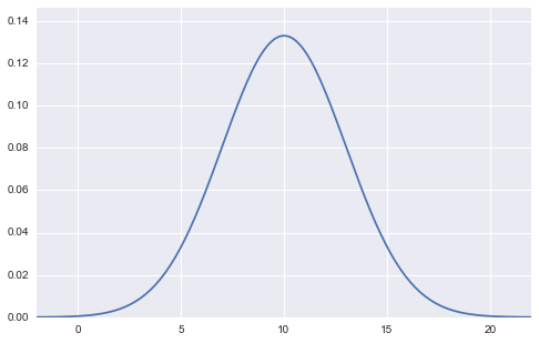
(Figure of normal distribution with mean 10 and standard deviation 3)

%matplotlib inline
import matplotlib.pyplot as plt
import matplotlib.cm as cm
import numpy as np
import seaborn as sns
import numpy.random as rd

m = 10
s = 3

min_x = m-4*s
max_x = m+4*s

x = np.linspace(min_x, max_x, 201)
y = (1/np.sqrt(2*np.pi*s**2))*np.exp(-0.5*(x-m)**2/s**2)

plt.figure(figsize=(8,5))
plt.xlim(min_x, max_x)
plt.ylim(0,max(y)*1.1)
plt.plot(x,y)
plt.show()

In this figure, the values of the two parameters, mean $ \ mu $ and standard deviation $ \ sigma $, are fixed (in the case of the above figure, mean $ \ mu = 10 $, standard deviation $ \ sigma = 3 $). , $ X $ is taken as a variable on the horizontal axis. The vertical axis as the output is the probability density $ f (x) $.

The basic concept of the likelihood function is to answer the question, "After sampling and observing the data, what parameters did the data originally come from?" So, I think there is an inversely probabilistic Bayes' theorem. (In fact, likelihood is a component of Bayes' theorem)

(Hereafter, the term data is referred to as a sample).

Here we get 10 samples ($ {\ bf x} = (x_1, x_2, \ cdots, x_ {10}) $), which we know follow a normal distribution, but mean $ \ mu Consider a situation where it is unclear what the values of the two parameters $ and standard deviation $ \ sigma $ are.

plt.figure(figsize=(8,2))
rd.seed(7)
data = rd.normal(10, 3, 10, )
plt.scatter(data, np.zeros_like(data), c="r", s=50)

First, let us consider the "joint distribution with 10 samples having this value". We also assume that these 10 samples are iid (independent identical distribution: samples taken independently from the same distribution). Since it is independent, it can be expressed as the product of each probability density.

P(x_1, x_2,\cdots,x_{10}) = P(x_1)P(x_2)\cdots P(x_{10})

It will be. Since $ P (x_i) $ was all normally distributed here,

P(x_1, x_2,\cdots,x_{10}) = f(x_1)f(x_2)\cdots f(x_{10})

It is also good. If you expand this further and write

P(x_1, x_2,\cdots,x_{10}) = \prod_{i=1}^{10} {1 \over \sqrt{2\pi\sigma^{2}}} \exp \left(-{1 \over 2}{(x_i-\mu)^2 \over \sigma^2} \right)

is. The specimen $ x_i $ is now inside $ \ exp (\ cdot) $.

You now have a simultaneous probability density function for 10 samples. But wait a minute. Now that the sample has a realization value, it is no longer an uncertain stochastic value. It is a fixed value. Rather, we didn't know the two parameters, mean $ \ mu $ and standard deviation $ \ sigma $. So, think of $ x_i $ as a constant, and change your mind to say that $ \ mu $ and $ \ sigma $ are variables.

The form of the function is exactly the same, and the variable re-declared as $ \ mu $ and $ \ sigma $ is defined as the likelihood.

L(\mu, \sigma) = \prod_{i=1}^{10} {1 \over \sqrt{2\pi\sigma^{2}}} \exp \left(-{1 \over 2}{(x_i-\mu)^2 \over \sigma^2} \right)

will do. The shape of the right side does not change at all. But the meaning has changed.

I will understand this as a graph.

Write and understand graphs

Since $ \ mu $ and $ \ sigma $ are unknown, if you think that $ \ mu = 0 $ and $ \ sigma = 1 $ and draw a graph,

It will be. It feels like it's completely removed. At this time, the likelihood is also small.

(Likelihood is calculated by multiplying the probability (density) by the number of samples, so the number between 0 and 1 will be multiplied many times, and the multiplication will be a fairly small number, almost 0. In many cases, the log-likelihood is used because of the ease of calculation that can be added. In that case, the value can be easily understood by looking at the value in the title of the above graph.)

m = 0
s = 1


min_x = m-4*s
max_x = m+4*s

def norm_dens(val):
    return (1/np.sqrt(2*np.pi*s**2))*np.exp(-0.5*(val-m)**2/s**2)
                                      
x = np.linspace(min_x, max_x, 201)
y = norm_dens(x)

L = np.prod([norm_dens(x_i) for x_i in data])
l = np.log(L)

plt.figure(figsize=(8,5))
plt.xlim(min_x, 16)
plt.ylim(-0.01,max(y)*1.1)

#Drawing the density function of the normal distribution
plt.plot(x,y)

#Drawing data points
plt.scatter(data, np.zeros_like(data), c="r", s=50)
for d in data:
    plt.plot([d, d], [0, norm_dens(d)], "k--", lw=1)
    
plt.title("Likelihood:{0:.5f}, log Likelihood:{1:.5f}".format(L, l))

plt.show()

Since the sample is located where the probability density function is almost 0, $ L (\ mu, \ sigma) $ also has a fairly small likelihood (log-likelihood: about -568).

Let's try $ \ mu = 5 $ and $ \ sigma = 4 $ this time. (The code is changed from the previous one only at $ \ mu = 5 $ and $ \ sigma = 4 $)

The dotted line shows the likelihood corresponding to each sample. It feels like it's getting a little warmer than before. This time, the log-likelihood is about -20, which is quite large.

Animate and be more intuitive

Let's animate how the likelihood changes as $ \ mu $ changes. You can see that the log-likelihood is maximized at $ \ mu = 10 $: grin:

from matplotlib import animation as ani

num_frame = 30

min_x = -11
max_x = 21

x = np.linspace(min_x, max_x, 201)

    
def norm_dens(val, m, s):
    return (1/np.sqrt(2*np.pi*s**2))*np.exp(-0.5*(val-m)**2/s**2)
    
def animate(nframe):
    global num_frame
    plt.clf()
    
    m = nframe/float(num_frame) * 15
    s = 3
    y = norm_dens(x, m, s)
    
    L = np.prod([norm_dens(x_i, m, s) for x_i in data])
    l = np.log(L)

    plt.xlim(min_x, 16)
    plt.ylim(-0.01,max(y)*1.1)

    #Drawing the density function of the normal distribution
    plt.plot(x,y)

    #Drawing data points
    plt.scatter(data, np.zeros_like(data), c="r", s=50)
    for d in data:
        plt.plot([d, d], [0, norm_dens(d, m, s)], "k--", lw=1)

    plt.title("mu:{0}, Likelihood:{1:.5f}, log Likelihood:{2:.5f}".format(m, L, l))

    #plt.show()
    
fig = plt.figure(figsize=(10,7))
anim = ani.FuncAnimation(fig, animate, frames=int(num_frame), blit=True)
anim.save('likelihood.gif', writer='imagemagick', fps=1, dpi=64)

When $ \ sigma $ changes, you can see that the log-likelihood is maximum when $ \ sigma = 2.7 $. When the data was originally generated, it was $ \ sigma = 3 $, so there is a slight error, but the values are close to each other: kissing_closed_eyes:

num_frame = 30

min_x = -11
max_x = 21

x = np.linspace(min_x, max_x, 201)
    
def norm_dens(val, m, s):
    return (1/np.sqrt(2*np.pi*s**2))*np.exp(-0.5*(val-m)**2/s**2)
    
def animate(nframe):
    global num_frame
    plt.clf()
    
    m = 10
    s = nframe/float(num_frame) * 5
    y = norm_dens(x, m, s)
    
    L = np.prod([norm_dens(x_i, m, s) for x_i in data])
    l = np.log(L)

    plt.xlim(min_x, 16)
    plt.ylim(-0.01,.6)

    #Drawing the density function of the normal distribution
    plt.plot(x,y)

    #Drawing data points
    plt.scatter(data, np.zeros_like(data), c="r", s=50)
    for d in data:
        plt.plot([d, d], [0, norm_dens(d, m, s)], "k--", lw=1)

    plt.title("sd:{0:.3f}, Likelihood:{1:.5f}, log Likelihood:{2:.5f}".format(s, L, l))

    #plt.show()
    
fig = plt.figure(figsize=(10,7))
anim = ani.FuncAnimation(fig, animate, frames=int(num_frame), blit=True)
anim.save('likelihood_s.gif', writer='imagemagick', fps=1, dpi=64)

Maximum likelihood estimation

It is a graph of the change in log-likelihood when $ \ mu $ is changed. You can see that the value of $ \ mu $ will be around 10 when the likelihood is differentiated by $ \ mu $ and set to 0. This is the maximum likelihood estimation. (Assuming that s is fixed for the time being)

#Change m

list_L = []
s = 3

mm = np.linspace(0, 20,300)
for m in mm:
    list_L.append(np.prod([norm_dens(x_i, m, s) for x_i in data]))
    

plt.figure(figsize=(8,5))
plt.xlim(min(mm), max(mm))
plt.plot(xx, (list_L))
plt.title("Likelihood curve")
plt.xlabel("mu")

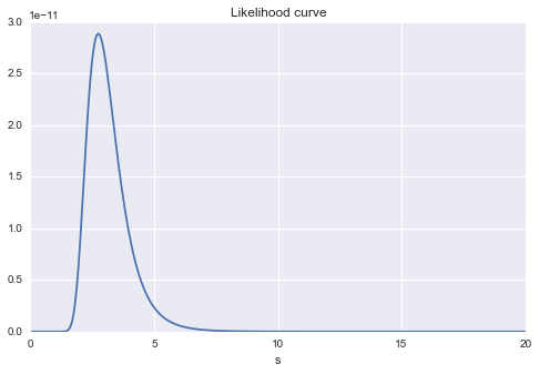
It is also a graph of the change in likelihood for changes in $ s $. You can still see that there is likely to be a maximum value around $ s = 3 $.

#Change s

list_L = []
m = 10

ss = np.linspace(0, 20,300)
for s in ss:
    list_L.append(np.prod([norm_dens(x_i, m, s) for x_i in data]))
    
plt.figure(figsize=(8,5))
plt.xlim(min(ss), max(ss))
plt.plot(ss, (list_L))
plt.title("Likelihood curve")
plt.xlabel("s")

Finally, if you look at $ \ mu $ and $ \ sigma $ at the same time, $ \ mu $ is a little more than 10 and $ \ sigma $ is a little less, and the maximum likelihood estimates are $ \ mu $ and $. You can see that the value of \ sigma $ is likely: satisfied:

#contour

plt.figure(figsize=(8,5))
mu = np.linspace(5, 15, 200)
s = np.linspace(0, 5, 200)
MU, S = np.meshgrid(mu, s)

Z = np.array([(np.prod([norm_dens(x_i, a, b) for x_i in data])) for a, b in zip(MU.flatten(), S.flatten())])
plt.contour(MU, S, Z.reshape(MU.shape), cmap=cm.Blues)
plt.xlabel("mu")
plt.ylabel("s")

[PYTHON] [Statistics] What is likelihood? Let's explain graphically.

Taking the normal distribution as an example

Write and understand graphs

Animate and be more intuitive

Maximum likelihood estimation