Introduction

** "I'm not so familiar with statistics, but I want to implement a model such as machine learning myself! 』** That is often the case, right?

Please be honest with those who think "There is no such thing (# ^ ω ^)". You must have thought about it once.

In particular, I think many people have wanted to implement logistic regression in Python **. ** There should be many **.

Here, we will implement a Logistic regression model that actually works in Python, explaining that the knowledge of statistics is null. Explanation of statistics ➔ Implementation can be advanced step by step so that even those who are not familiar with statistics can do it without difficulty.

For some reason, it is efficient to learn statistical models and machine learning while implementing them yourself.

Target audience for this article

Basically, it is for those who are a little interested in data science.

――I've heard about logistic regression, but I'm not sure. --My boss is noisy to classify with logistic regression ――I'm not familiar with statistics, but I feel like I can learn while implementing it. ――I have the minimum knowledge, but I want to know how it works ――Of course you have used logistic regression? It's a package. Actually, I haven't implemented it myself, but /// What are you complaining about?

I want to read it together

If you are interested in data scientists, first look around here, a summary of literature and videos http://qiita.com/hik0107/items/ef5e044d2f47940ba712

It's time to seriously think about the definition and skill set of data scientists http://qiita.com/hik0107/items/f9bf14a7575d5c885a16

Preparation

Make the following settings.

import numpy as np
import pandas as pd
import matplotlib.pyplot  as plt
from scipy import optimize

plt.style.use('ggplot')

Also, it may be better to study only the outline of logistic regression in this article. (It's okay if you can understand the atmosphere somehow.) http://gihyo.jp/dev/serial/01/machine-learning/0018

Implementation

Generate data

This time, for the sake of simplicity, we will create data with only two elements and binary classification. Let $ x, y $ be an element and $ c = [1,0] $ be a binary classification. Let's create a function that generates $ N points $ for this combination and stores it in a Pandas Data Frame.

$ obs_i = (x_i, y_i, c_i) $ where $ i = 1,2,3 .... N $

$ x_i and y_i $ can be easily created with the numpy module "np.random".

For $ c $, we will artificially define a separation line and allocate it according to which side of the separation line it is on. Let's assume that the separator line is $ 5x + 3 y = 1 $. That is, $ g (x, y) = 5x_i + 3y_i -1 $, $ g (x, y)> 0 ⇛ c = 1 $, $ g (x, y) <0 ⇛ c = 0 $ To

`make_data.py`



def make_data(N, draw_plot=True, is_confused=False, confuse_bin=50):
    '''A function that generates N datasets
Function to intentionally complicate data is_Implement confused
    '''
    np.random.seed(1) #Fix the seed so that the random numbers have the same output each time
    
    feature = np.random.randn(N, 2)
    df = pd.DataFrame(feature, columns=['x', 'y'])

    #Binary classification: Mechanically determine whether you are above or below the artificial separation line
    df['c'] = df.apply(lambda row : 1 if (5*row.x + 3*row.y - 1)>0 else 0,  axis=1)

    #Disturbance:Operations to make the data a little more complicated
    if is_confused:
        def get_model_confused(data):
            c = 1 if (data.name % confuse_bin) == 0 else data.c 
            return c

        df['c'] = df.apply(get_model_confused, axis=1)
    
    #Visualization: A module that visualizes what the data looks like
    # c = df.c In other words, the two values 0 and 1 are displayed separately in color.
    if draw_plot:
        plt.scatter(x=df.x, y=df.y, c=df.c, alpha=0.6)
        plt.xlim([df.x.min() -0.1, df.x.max() +0.1])
        plt.ylim([df.y.min() -0.1, df.y.max() +0.1])
        
    return df

Let's look at the output of this function

`make_data.py`


df = make_data(1000)
df.head(5)

Out[24]:
        x           y       c
0	1.624345	-0.611756	1
1	-0.528172	-1.072969	0
2	0.865408	-2.301539	0
3	1.744812	-0.761207	1
4	0.319039	-0.249370	0

You can see that c = 1 and c = 0 are separated by a certain line in Sakai.

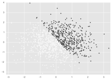
This is the $ 5x + 3 y = 1 $ line defined above. It is successful if the Logistic regression model to be implemented can predict this separation line.

This time, I added a little extra to this data generation function.

`make_data.py`


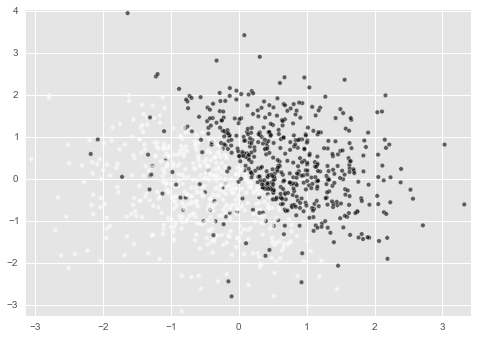
df_data = make_data(1000, is_confused=True, confuse_bin=10)

By specifying the argument in this way, it is possible to mix the black spots in the white spot area. The amount of mixing is set to increase as confuse_bin becomes smaller. I'll see what this means later (though some of you may already know).

Calculate the probability value

** The advantage of logistic regression is that "the probability that c = 1 can be considered" is output as a probability value of $ 0 ≤ p ≤ 1 $ **, so that each data is ** which The point is that it is possible to clarify ** which of the two values of $ [1, 0] $ is classified with a certain degree of certainty.

So, next we will implement the calculation of this probability value p. This is easy if you put the theoretical side aside. Let's start with the conclusion code.

`make_data.py`


def sigmoid(z):
    return 1.0 / (1 + np.exp(-z))


def get_prob(x, y, weight_vector):
    '''Given the features and the weighting factor vector, the probability p(c=1 | x,y)Function that returns
    '''
    feature_vector =  np.array([x, y, 1])
    z = np.inner(feature_vector, weight_vector)
    
    return sigmoid(z)

that's all. It's that easy, isn't it? I will supplement it a little. (If you are interested in theory, you can find a lot of information by google.)

The probability that an observation point is classified as $ c = 1 $ $ p (c = 1 | x) $ is described as follows.

$ p = \ frac {1} {1 + exp (-f)} $ where $ f = ∑ w_iφ (x_i) $

In this case, $ f = w_1x + w_2y + w_3 $. Where $ w_1, w_2, w_3 $ refer to parameters called ** weights **.

In short, it refers to the slope or intercept of the line on the x-y axis graph.

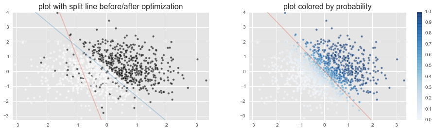
In this figure, the red line does not separate ** c = 1 and c = 0 (black and white) well **, isn't it? This is because each weight, such as $ w_1, w_2, w_3 $, is incorrect as a model for classifying this data.

I don't like this red line, so I want to see the blue line ** It seems that c = 1 and c = 0 (black and white) can be separated well ** Searching for weights is called "creating a logistic regression model" It corresponds to that.

Well, it looks easy.

Let's find the best "weight"

I'm going to beat it a little from here. ** Everyone loves maximum likelihood estimation **. Likelihood can be described as follows with the weight vector $ w $ as a parameter.

$ E(w) = ∑- log(L_i) $

However, the likelihood $ L_i $ of an observation point with $ c_i = [1, 0] $ as the correct answer is defined as follows. As mentioned above, $ p_i $ is a function of $ w $.

$L_i = c_i log (p_i) +(1-c_i) log(1-p_i) $

I'm saying something that seems difficult, but it's not that difficult. Think of it this way.

There are three points, and the classification value of these points is $ (c_1, c_2, c_3) = (1,1,0) $. Black Black White.

Now, let's say you have two predictive models created by logistic regression. Each model predicted the probability that these three points would be 1 (black) as follows: ** Which is the better model **?

M_1 : (p_1,p_2,p_3) = (0.8, 0.6, 0.2) M_2 : (p_1,p_2,p_3) = (0.9, 0.1, 0.1)

Intuitively (1) Think about how well the predictions for each point (1 to 3) are correct. ② Considering the sum of the three Overall, I feel like I can say how good and good the predictions are.

Statistically, I think as follows. For example, in the example of $ M_1 $

$ p_1 $ is $ correct answer: for c = 1 $, it is predicted to be ** 0.8 **, so 0.8 points $ p_2 $ predicts ** 0.6 ** for $ correct answer: c = 1 $, so 0.6 points $ p_3 $ predicts ** 0.2 ** for $ correct answer: c = 0 $, so (1.0-0.2) = 0.8 points

The total score shall be 0.8, 0.6, 0.8 multiplied by ** **.

Note that $ p_3 $ is not 0.2 points

In this way, if you compare the scores of $ M_1 $ and $ M_2 $, you can compare which model is better.

Actually, when predicting with N point data, it is a product of the predictions of $ p_1, p_2 ... p_N $. Also, instead of looking for two models, look for the best one out of the myriad of possibilities.

Perhaps there are many questions in this regard. For more information, please go to "Maximum likelihood estimation Saiyusuite".

Q. Why do you ** multiply the scores **? A. Because it's a probability

Q. What is $ log $ in the above formula? A. $ log $ has advantages such as being able to convert multiplication to addition.

Q. If you do $ log $ without permission, the meaning of the expression will change. What's the minus? A. The maximization of the value taken by $ log $ matches the maximization of the original value. A. Replacing the maximization problem with the minimization problem> Minus

Q. How do you find the best ** out of the myriad of possibilities? A. We'll cover it in the next chapter, but it doesn't go into too much detail.

Find the weight: Maximum likelihood estimation

First, implement the likelihood you want to optimize. Again, the likelihood of a model (= a weight $ w_1, w_2, w_3 $) is formulated as follows, so I'm just coding it.

$ E(w) = ∑- log(L_i) $
However, $ L_i = c_i log (p_i) + (1-c_i) log (1-p_i) $

`estimate_param.py`


def define_likelihood(weight_vector, *args):
    '''A function that defines the sum of log-likelihoods by licking the df dataset
Feed this function to Optimizer to estimate the maximum likelihood of parameters
    '''
    likelihood = 0
    df_data = args[0]
    
    for x, y, c in zip(df_data.x, df_data.y, df_data.c):
        prob = get_prob(x, y, weight_vector)

        i_likelihood = np.log(prob) if c==1 else np.log(1.0-prob)
        likelihood = likelihood - i_likelihood
        
    return likelihood

Then, find the weights $ w_1, w_2, w_3 $ that give the best likelihood defined in the above code. Avoid self-implementation here, and leave it to scipy.optimize, a package for finding minimization solutions for functions.

`estimate_param.py`


def estimate_weight(df_data, initial_param):
    '''Receive the training data and the initial values of the parameters,
A function that returns the optimal parameters of the maximum likelihood estimation result
    '''        
    parameter = optimize.minimize(define_likelihood,
                                  initial_param, #Give the initial value of the appropriate weight combination
                                  args=(df_data),
                                  method='Nelder-Mead')
    
    return parameter.x

Like I did here

The result of classification is represented by elements ($ x $ or $ y $) x their weights $ w_1, w_2, w_3 $

Express the likelihood as a function of weights

Find a combination of weights that optimizes the likelihood

This flow is very common in the world of statistical models and machine learning. I think it's worth remembering.

Now let's run the implemented function to find the optimal weight.

First, define the initial value of the weight appropriately. This is perfectly appropriate.

Depending on the optimization problem, the result may change depending on the initial value, but here it is appropriate and okay.

`optimize.py`


weight_vector = np.random.rand(3)
weight_vector

Out[26]:
array([ 0.91726016,  0.15073966,  0.24376398])

`optimize.py`


#Create data and plot
df_data = make_data(1000)

#Set an appropriate initial weight and try drawing the separation surface
weight_vector = np.random.rand(3)
draw_split_line(weight_vector)

Here, I made the following function to draw the separation surface.

`draw_split_line.py`


def draw_split_line(weight_vector):
    '''Function to draw a separator line
    '''
    a,b,c = weight_vector
    x = np.array(range(-10,10,1))
    y = (a * x + c)/-b
    plt.plot(x,y, alpha=0.3)

The result looks like this. I pulled it properly, so it's obviously off the mark.

Now, let's find a nice weight so that we can separate white and black well.

`optimize.py`


weight_vector = estimate_weight(df_data, weight_vector) #Executing maximum likelihood estimation
weight_vector

Out[30]:
array([ 10013.66435446,   6084.79071201,  -2011.60925704])

The optimal weight has been found. Now, remember that the separation plane we defined this time was $ 5x + 3 y = 1 $. Can you see that the weights $ (w_1, w_2, w_3) $ are close to $ (5: 3: -1) $?

If you draw a line with draw_split_line (), it will look like the figure below. Overflowing ** Feeling good at it **

What happened to the probability p of c = 1

I have a rest. For the time being, implement the following function.

`predict.py`


def validate_prediction(df_data, weight_vector):
    
    a, b, c = weight_vector
    df_data['pred'] = df_data.apply(lambda row : 1 if (a*row.x + b*row.y + c) >0 else 0, axis=1)
    df_data['p'] = df_data.apply(lambda row :  sigmoid(a*row.x + b*row.y + c), axis=1)
        
    return df_data

** "pred" ** is the predicted value when the point where P = 0.5 or more is predicted as c = 1. ** "p" ** is the predicted value of the probability that c = 1.

df_pred = validate_prediction(df_data, weight_vector)
df_pred.head(10)

Out[33]:
        x	        y	   c	pred	  p
0	1.624345	-0.611756	1	1	1.000000e+00
1	-0.528172	-1.072969	0	0	0.000000e+00
2	0.865408	-2.301539	0	0	0.000000e+00
3	1.744812	-0.761207	1	1	1.000000e+00
4	0.319039	-0.249370	0	0	7.043082e-146
5	1.462108	-2.060141	1	1	1.000000e+00
6	-0.322417	-0.384054	0	0	0.000000e+00
7	1.133769	-1.099891	1	1	1.000000e+00
8	-0.172428	-0.877858	0	0	0.000000e+00
9	0.042214	0.582815	1	1	1.000000e+00

Since the actual value of c and the value of pred match, is the prediction successful? If you are interested, please check all 1000 data.

Also, the probability value p is required. It is a characteristic of logistic regression that you can get this $ p $ instead of simply spitting out either 1,0 answer. Let's see what p looks like.

`show_p.py`


def draw_prob(df_data):

    df = validate_prediction(df_data, weight_vector)
    plt.scatter(df_data.x, df_data.y, c=df_data.p, cmap='Blues', alpha=0.6)
    plt.xlim([df_data.x.min() -0.1, df.x.max() +0.1])
    plt.ylim([df_data.y.min() -0.1, df.y.max() +0.1])
    plt.colorbar()
    
    plt.title('plot colored by probability', size=16)

I made an appropriate function to visualize $ p $ like this.

Since it's a big deal, I will use the function created so far and execute it through the whole flow.

`run_predict.py`


plt.figure(figsize=(16, 4))
plt.subplot(1,2,1) #Preparing to display two figures side by side

#Create data and plot
df_data = make_data(1000)

#Set an appropriate initial weight and try drawing the separation surface
weight_vector = np.random.rand(3)
draw_split_line(weight_vector)

#Estimate the weight by maximum likelihood estimation and try drawing the separation surface
weight_vector = estimate_weight(df_data, weight_vector)
draw_split_line(weight_vector)
plt.title('plot with split line before/after optimization', size=16)

#Visualization of p
plt.subplot(1,2,2)
draw_prob(df_data)

You can see that the probability p (degree of blueness in the figure on the right) that c = 1 is clearly divided on the separation surface in Sakai. This is because the data itself was such that c = 1 or 0 was clearly separated above and below the separation surface.

As the word says, it's ** black and white clearly **. In the actual data, the value of c will not be separated so beautifully.

Try with a little more complicated data

So, let's try with a little more complicated data. Recall the data above.

In reality, even data in the same area like this usually has c = 1 or c = 0. What happens in this case?

`run_predict.py`


plt.figure(figsize=(16, 4))
plt.subplot(1,2,1)

#Create data and plot(Only here is different)
df_data = make_data(1000,is_confused=True, confuse_bin=10)

#Set an appropriate initial weight and try drawing the separation surface
weight_vector = np.random.rand(3)
draw_split_line(weight_vector)

#Estimate the weight by maximum likelihood estimation and try drawing the separation surface
weight_vector = estimate_weight(df_data, weight_vector)
draw_split_line(weight_vector)

plt.title('plot with split line before/after optimization', size=16)

plt.subplot(1,2,2)
draw_prob(df_data)
#draw_split_line(weight_vector)

The results have changed a lot. In the figure on the left, the position of the separation surface is slightly closer to the white catamari group, and in the figure on the right, the color near the separation surface is moody.

This means that ** the model is not black and white clear because the data is not black and white clearer than before **.

The idea of logistic regression is to judge c = 1 when this blue is ◯◯ or more (for example, 0.6 or more).

Summary

--Implemented logistic regression in Python --I somehow learned about the theory of logistic regression ――I feel confident that I can make a classification model for machine learning by myself.

The first step for those who are amateurs of statistics but want to implement machine learning models in Python

** Introduction **

** Target audience for this article **

** I want to read it together **

** Preparation **

Implementation

** Generate data **

make_data.py

make_data.py

make_data.py

** Calculate the probability value **

make_data.py

** Let's find the best "weight" **

** Find the weight: Maximum likelihood estimation **

estimate_param.py

estimate_param.py

optimize.py

optimize.py

draw_split_line.py

optimize.py

** What happened to the probability p of c = 1 **

predict.py

show_p.py

run_predict.py

** Try with a little more complicated data **

run_predict.py

** Summary **

Introduction

Target audience for this article

I want to read it together

Preparation

Generate data

`make_data.py`

`make_data.py`

`make_data.py`

Calculate the probability value

`make_data.py`

Let's find the best "weight"

Find the weight: Maximum likelihood estimation

`estimate_param.py`

`estimate_param.py`

`optimize.py`

`optimize.py`

`draw_split_line.py`

`optimize.py`

What happened to the probability p of c = 1

`predict.py`

`show_p.py`

`run_predict.py`

Try with a little more complicated data

`run_predict.py`

Summary