Try building a neural network in Python without using a library
Code here: All code is also available on Ipython Notebook on Github.
In this post, we will build a simple neural network with 1 to 3 layers. I will not explain all the mathematics that comes out, but I would like to explain the necessary parts in an easy-to-understand manner. If you are interested in the details of mathematics, most of them are in English, but here are some helpful links.
- It is assumed that the readers of this post know at least the basics of differentiation and machine learning (classification, regularization, etc.). It's even better if you know optimization techniques like Gradient Descent. However, even if you don't know the above, I think that anyone who is interested in neural networks can enjoy it.
So why do we need to build a neural network from scratch without using a library? I plan to use neural network libraries like PyBrain and Tensorflow in a later post, for the reason. The experience of building a neural network from scratch even once is extremely valuable. Let's design a model by knowing how a neural network works and is built! It is useful at such times.
One caveat is that the code below isn't written efficiently because this post focuses on comprehension. I will explain how to write efficient code in a later post. In that case, use Theano.
Generate data
Now, let's generate the data first. Luckily, Scikit-learn has a dataset generation kit that you can use, so you don't have to write your own code. This time, let's use the make_moons function to create moon-shaped data.
#Generate and plot data
np.random.seed(0)
X, y = sklearn.datasets.make_moons(200, noise=0.20)
plt.scatter(X[:,0], X[:,1], s=40, c=y, cmap=plt.cm.Spectral)

There are two classes of generated data (red and blue dots on the graph). For example, consider the blue dots as male patient data samples and the red dots as female patient data samples, and the X and Y axes as specific measurements.
Our goal is to machine-learn the classification model to predict and give the correct class for each sample point. It should be noted that this data cannot be classified by a straight line. Therefore, with Linear Classifiers like logistic regression, you can't make a good model unless you make your own non-linear features such as polynomials. However, for this data, it is possible to create a good model by leading the polynomial characteristics.
Leading a neural network can solve this problem. Because you don't have to do Feature Engineering. The hidden layer of the neural network finds the characteristics.
Logistic regression
Before explaining the neural network, let's first train the logistic regression model. The input data is a point on the X / Y axis and the output data is its class (0 or 1). Since this is a preparation for the explanation of the neural network below, let's build a logistic regression model using schikit-learn.
#Train a logistic regression model
clf = sklearn.linear_model.LogisticRegressionCV()
clf.fit(X, y)

#Plot the decision boundaries
plot_decision_boundary(lambda x: clf.predict(x))
plt.title("Logistic Regression")

In the graph directly above, the logistic regression model is trained and the classes are classified with the Decision Boundary as the boundary. This boundary line leads a straight line and classifies as much as possible, but it does not recognize the "moon shape" of the data.
Train a neural network
Now, let's build a 3-layer neural network (1 input layer, 1 hidden layer, 1 output layer). The number of nodes in the input layer (circle in the figure below) is the number of dimensions of the data (2 this time). And the number of nodes in the output layer is the number of classes, this time also 2 (By the way, since it is 2 classes, it is possible to make one of 1 or 0 an output node, but later multiple classes This time we will use two nodes in consideration of dealing with). The input of the network is the point (X, Y) and the output is the probability of being either class 0 (female) or class 1 (male). Please refer to the figure below.

Next, determine the dimension of the hidden layer (the number of nodes). As the number of hidden layer nodes increases, more complex models can be built. On the other hand, as the number of nodes increases, computing power is required to learn and predict parameters. It is also important to note that the risk of overfitting increases as the number of parameters increases.
How do you choose the number of hidden layers? Although there are general guidelines, the choices are on a case-by-case basis and should be considered more like art than science. Below, we'll try a few different numbers of hidden layer nodes to see how they affect the output.
Another thing to decide is the hidden layer activation function. This is a function to transform the input data and output it. You can train nonlinear data by leading a nonlinear activation function. Common examples of activation functions are Tanh, [Sigmoid Function](https://en.wikipedia.org/wiki/ Sigmoid_function), and ReLUs. This time, I will use tanh, which can produce relatively good results in various cases. A convenient property of this function is that you can calculate the derivative by leading the original value. For example, the derivative of $ tanhx $ is $ 1-tanh ^ 2x $. Therefore, once $ tanhx $ is calculated, it can be reused later.
This time, we want to give a probability to the output, so we will use the Softmax function for the activation function of the output layer. You can convert non-probable numbers to probabilities by leading this function. If you are familiar with the logistic regression model, think of the Softmax function as a generalized version of multiple classes.
Neural network prediction mechanism
This neural network uses a kind of matrix multiplication called forward propagation and an application of the activation function defined above. If the input x is 2D, the predicted value $ \ hat {y} $ (also 2D) is calculated as follows.
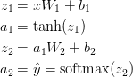
$ z_i $ is the input layer i, and $ a_i $ is the output layer i converted by the activation function. $ W_1 $, $ b_1 $, $ W_2 $, $ b_2 $ are network parameters that need to be learned from the training data. You can think of it as a matrix transformation between network layers. If you look at the matrix multiplication above, you can see the number of dimensions of the matrix. For example, if you use 500 hidden nodes, $ W_1 \ in \ mathbb {R} ^ {2 \ times 500} $, $ b_1 \ in \ mathbb {R} ^ {500} $, $ W_2 \ in \ mathbb {R } ^ {2 \ times 500} $, $ b_2 \ in \ mathbb {R} ^ {2} $. So you can see why increasing the size of the hidden layer increases the parameters.
Train parameters
Training the parameters means looking for the parameters ($ W_1 $, $ b_1 $, $ W_2 $, $ b_2 $) that minimize the error value on the training data. So how do you define the error value? The function that measures the error value is called the Loss function. For Softmax, the commonly used Loss function [Minimize Cross Entropy](https://ja.wikipedia.org/wiki/%E4%BA%A4%E5%B7%AE%E3%82%A8%E3 Leads% 83% B3% E3% 83% 88% E3% 83% AD% E3% 83% 94% E3% 83% BC) (also known as negative log likelihood). If there is N learning data and there is C class, the Loss function of the predicted value $ \ hat {y} $ can be written as follows for the correct answer value y.

This method may seem complicated, but its role is as simple as adding the training data together and adding the value to Loss when the class is predicted by mistake. Therefore, the farther the two probability distributions, the predicted value $ \ hat {y} $ and the correct value y, are, the larger the Loss. Therefore, looking for a parameter that minimizes Loss is the same as maximizing the likelihood of the training data.
Use Gradient Descent to calculate the minimum Loss value. This time I will lead a simple batch gradient descent (learning rate is constant), but [stochastic gradient descent](https://ja.wikipedia.org/wiki/%E7%A2%BA%E7%8E%87% E7% 9A% 84% E5% 8B% BE% E9% 85% 8D% E9% 99% 8D% E4% B8% 8B% E6% B3% 95) and mini-batch gradient descent would be more practical. It is also more practical to gradually reduce the learning rate.
Gradient descent parameters ($ \ frac {\ partial {L}} {\ partial {W_1}} $, $ \ frac {\ partial {L}} {\ partial {b_1}} $, $ \ frac { Calculate the gradient (differential value of the vector) of the Loss function for \ partial {L}} {\ partial {W_2}} $, $ \ frac {\ partial {L}} {\ partial {b_2}} $) is needed. We use the back-propagation algorithm to calculate this slope. This algorithm is an efficient way to calculate the slope from the output. Those who are interested in this mathematical commentary are here and [here](http://cs231n.github.io/optimization- Please read the explanation of 2 /).
Using back-propagation, the following holds.

Actually write the code
Let's finish the academic knowledge so far and actually write the code! First, let's set the variables and parameters for gradient descent.
 num_examples = len(X) #Data size for training
 nn_input_dim = 2 #Number of dimensions of the input layer
 nn_output_dim = 2 #Number of dimensions of the output layer

# Gradient descent parameters (Use commonly used values)
 epsilon = 0.01 #Gradient descent learning rate
 reg_lambda = 0.01 #Strength of regularization
Let's write the Loss function defined above. You can lead this to check the performance of your model.
#Helper function to calculate all Loss
def calculate_loss(model):
    W1, b1, W2, b2 = model['W1'], model['b1'], model['W2'], model['b2']
    #Forward propagation for calculating forecasts
    z1 = X.dot(W1) + b1
    a1 = np.tanh(z1)
    z2 = a1.dot(W2) + b2
    exp_scores = np.exp(z2)
    probs = exp_scores / np.sum(exp_scores, axis=1, keepdims=True)
    #Calculate Loss
    corect_logprobs = -np.log(probs[range(num_examples), y])
    data_loss = np.sum(corect_logprobs)
    #Give Loss a reguratization term(optional)
    data_loss += reg_lambda/2 * (np.sum(np.square(W1)) + np.sum(np.square(W2)))
    return 1./num_examples * data_loss
Write a Helper function to calculate the output layer. Leads the forward propagation described above and returns the highest probability.
# Helper function to predict an output (0 or 1)
def predict(model, x):
    W1, b1, W2, b2 = model['W1'], model['b1'], model['W2'], model['b2']
    # Forward propagation
    z1 = x.dot(W1) + b1
    a1 = np.tanh(z1)
    z2 = a1.dot(W2) + b2
    exp_scores = np.exp(z2)
    probs = exp_scores / np.sum(exp_scores, axis=1, keepdims=True)
    return np.argmax(probs, axis=1)
Finally, write the code to generate the neural network. Write the batch gradient descent using the backpropagation derivative described above.
# This function learns parameters for the neural network and returns the model.
# - nn_hdim: Number of nodes in the hidden layer
# - num_passes: Number of passes through the training data for gradient descent
# - print_loss: If True, print the loss every 1000 iterations
def build_model(nn_hdim, num_passes=20000, print_loss=False):

    # Initialize the parameters to random values. We need to learn these.
    np.random.seed(0)
    W1 = np.random.randn(nn_input_dim, nn_hdim) / np.sqrt(nn_input_dim)
    b1 = np.zeros((1, nn_hdim))
    W2 = np.random.randn(nn_hdim, nn_output_dim) / np.sqrt(nn_hdim)
    b2 = np.zeros((1, nn_output_dim))

    # This is what we return at the end
    model = {}

    # Gradient descent. For each batch...
    for i in xrange(0, num_passes):

        # Forward propagation
        z1 = X.dot(W1) + b1
        a1 = np.tanh(z1)
        z2 = a1.dot(W2) + b2
        exp_scores = np.exp(z2)
        probs = exp_scores / np.sum(exp_scores, axis=1, keepdims=True)

        # Backpropagation
        delta3 = probs
        delta3[range(num_examples), y] -= 1
        dW2 = (a1.T).dot(delta3)
        db2 = np.sum(delta3, axis=0, keepdims=True)
        delta2 = delta3.dot(W2.T) * (1 - np.power(a1, 2))
        dW1 = np.dot(X.T, delta2)
        db1 = np.sum(delta2, axis=0)

        # Add regularization terms (b1 and b2 don't have regularization terms)
        dW2 += reg_lambda * W2
        dW1 += reg_lambda * W1

        # Gradient descent parameter update
        W1 += -epsilon * dW1
        b1 += -epsilon * db1
        W2 += -epsilon * dW2
        b2 += -epsilon * db2

        # Assign new parameters to the model
        model = { 'W1': W1, 'b1': b1, 'W2': W2, 'b2': b2}

        # Optionally print the loss.
        # This is expensive because it uses the whole dataset, so we don't want to do it too often.
        if print_loss and i % 1000 == 0:
          print "Loss after iteration %i: %f" %(i, calculate_loss(model))

    return model
Neural network with 3 hidden layers
Now let's create a network with three hidden layers.
#Build a model with a 3D hidden layer
model = build_model(3, print_loss=True)

#Plot the decision boundaries
plot_decision_boundary(lambda x: predict(model, x))
plt.title("Decision Boundary for hidden layer size 3")

I recognized the moon shape well! You can divide the classes properly by the neural network.
Check the compatible size of the hidden layer
In the above, I chose 3 hidden layers. Below, let's compare while changing the number of hidden layers.
plt.figure(figsize=(16, 32))
hidden_layer_dimensions = [1, 2, 3, 4, 5, 20, 50]
for i, nn_hdim in enumerate(hidden_layer_dimensions):
    plt.subplot(5, 2, i+1)
    plt.title('Hidden Layer size %d' % nn_hdim)
    model = build_model(nn_hdim)
    plot_decision_boundary(lambda x: predict(model, x))
plt.show()
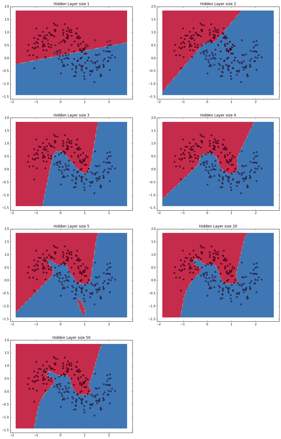
Looking at the figure above, we have a good grasp of the pattern of data for low-dimensional hidden layers (per 3,4). On the other hand, it seems that there is a risk of overfitting in higher dimensions. When that happens, it's like memorizing the data in its entirety rather than capturing the true shape of the data. If you lead the test data to check the model, you should be able to predict more accurately that it is a low-dimensional hidden layer. It would be more (computer-wise) "economical" to choose the right size hiding layer than to strongly regularize the overfit.
Well, this time I tried to create a network from scratch without using a library. Next, I will explain deep learning more deeply using the neural network library.
- Written with Denny Britz, who writes the wildML blog
Recommended Posts