Last time, I took up the pedestrian space network as an example of network analysis in architecture and cities, and actually drew the pedestrian space network with Rhinoceros based on the map information. → Read the network modeled by Rhinoceros in Python ①

The purpose of this article is to make the drawn network into a form that can be analyzed.

Goal

Draw a network with Rhinoceros
Export the network drawn in Rhinoceros so that it can be read in Python
Read the exported file with Python and create an adjacent array

This article addresses Section 2.

Adjacent array

Data structures that represent networks include adjacency matrices, distance matrices, and adjacency arrays. In this article, I will show you how to represent a network as an adjacent array.

Before that, a brief description of each data structure is given below.

** ・ Adjacency matrix ** A square matrix that represents the adjacency of ordered nodes as 0/1 (not adjacent/adjacent) is called an adjacency matrix. Strictly speaking, a graph that focuses only on the adjacency of nodes without considering the weight of the edges is called a ** graph **.

For example 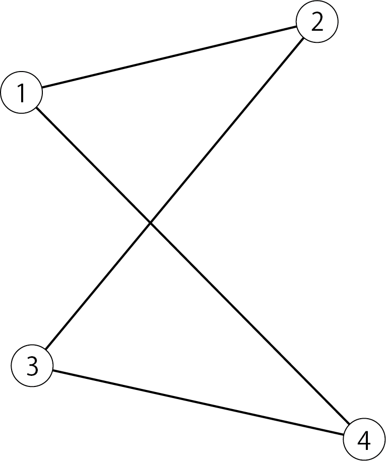Is represented by an adjacency matrix

\begin{pmatrix}
0&1&0&1\\
1&0&1&0\\
0&1&0&1\\
1&0&1&0
\end{pmatrix}

Will be.

By using the adjacency matrix, you can algebraically find the number of routes from node to node. The adjacency matrix is symmetric because the upper graph has no orientation at the edges (undirected graph), but it is also possible to break the symmetry and express a one-way edge (directed graph).

** ・ Distance matrix ** Each component of the adjacency matrix represented the adjacency between nodes. The distance matrix is the element given the weight of the edge connecting the nodes. A network that weights the edges of the graph above 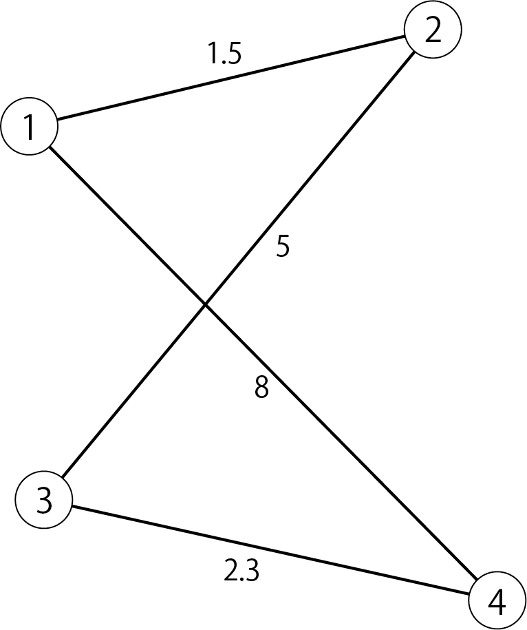Distance matrix is

\begin{pmatrix}
0&1.5&0&8\\
1.5&0&5&0\\
0&5&0&2.3\\
8&0&2.3&0
\end{pmatrix}

Will be. Note that we have placed 0s on the elements between non-adjacent nodes for convenience, but this does not mean that the edge weights are 0.

** ・ Adjacent array ** Both of the above two data structures use matrices. Now, if you think about networks in architecture and cities, you can imagine that there are at most four or five nodes adjacent to a node. At that time, the adjacency matrix and the distance matrix become a lot of 0s, which is very wasteful. Therefore, the adjacent array is to remember only the relationship between adjacent nodes.

If you actually create an adjacent array of the network, it will be as follows.

\begin{align}
&1: &[2, 4]\\
&2: &[1, 3]\\
&3: &[2, 4]\\
&4: &[1, 3]
\end{align}

An array of nodes of interest to the left of the colon and adjacent nodes to the right is shown. At the same time, remember the edge weights in the same way. This is tentatively called a distance array.

\begin{align}
&1: &[1.5, 8]\\
&2: &[1.5, 5]\\
&3: &[5, 2.3]\\
&4: &[8, 2.3]
\end{align}

Notice that the order of the adjacent array and the distance array correspond. By this correspondence, "It can be seen from the adjacent array that node 3 and node 2 are adjacent. The weight of the edge is 1 in the distance array of node 3 because node 2 is the first in the adjacent array of node 3. You can search for something like "Look at the second and see that it is 5."

Adjacent arrays allow you to remember large networks in a good way. Depending on the analysis you want to do and the analysis you want to do, you may need an adjacency matrix or a distance matrix, but for the time being, an adjacency array seems to be sufficient.

Export the modeled network as an adjacent array

Now, let's finally make the network modeled by Rhinoceros an adjacent array. The environment is Windows 10, Rhinoceros 5.

Method

The code below requires that the network be all modeled in straight lines.

First, in the Rhinoceros command,

EditPythonScript

Start the Python editor, paste the following code, and run it. The part labeled check point will be explained later.

`rhino_network_write.py`


# coding utf-8

import rhinoscriptsyntax as rs

import math
import random
import sys
import os

""" check point1 """
edges = rs.GetObjects("select objects")

adjacentList = {}
attributeList = {}
""" check point2 """
coordinations = []
coordinations_rounded = []  # for checking if a point is searched already or not

"""
example
adjacentList =  {0: [1, 2, 3], 1: [0, 2],...}
attributeList = {0: [2.0, 5.0, 8.6], 1: [2.0, 4.7], ...}
coordinations = [[4.5, 8.2, 0.0], [5.2, 3.6, 0.0], ...]
"""

cnt = 0   # point id
for i in range(len(edges)):
    edge = edges[i]
    try:
        end_points = rs.CurvePoints(edge)
    except:
        rs.ObjectColor(edge, (255, 0, 0))
        print("Error", edge)
        break
    
    l = rs.CurveLength(edge)
    """ check point3 """
    kind = rs.ObjectLayer(edge)
    
    for p in end_points:
        """ check point4 """
        p_rounded = [round(p[0], 2), round(p[1], 2), round(p[2], 2)] # round to the second decimal place
        if p_rounded in coordinations_rounded: # this point is already searched
            pass
        else: # search a new point 
            coordinations.append(p)
            coordinations_rounded.append(p_rounded)
            adjacentList[cnt] = []
            attributeList[cnt] = []
            cnt += 1
            
    # two end points are connected
    point_ids = [coordinations_rounded.index([round(p[0], 2), round(p[1], 2), round(p[2], 2)]) for p in end_points]
    
    adjacentList[point_ids[0]].append(point_ids[1])
    adjacentList[point_ids[1]].append(point_ids[0])
    
    attributeList[point_ids[0]].append((l, kind)) # you can add another info in attributeList
    attributeList[point_ids[1]].append((l, kind))

for k in adjacentList.keys():
    rs.AddTextDot(k, coordinations[k])

# set your path to the project folder
f = open("C:\\Users\\Owner\\Desktop\\adjacentList.txt", "w")
for k, v in adjacentList.items():
    print(k, v)
    f.write(str(k)+"\n")
    for nei in v:
        f.write(str(nei)+",")
    f.write("\n")
f.close()

f = open("C:\\Users\\Owner\\Desktop\\attributeList.txt", "w")
for k, v in attributeList.items():
    print(k, v)
    f.write(str(k)+"\n")
    for ats in v:   #ats = (length, layer_name)
        for at in ats:
            f.write(str(at)+"\n")
    f.write("_\n")
f.close()

f = open("C:\\Users\\Owner\\Desktop\\coordinations.txt", "w")
for p in coordinations:
    for u in p:
        f.write(str(u)+"\n")
f.close()

When the code finishes running, you'll get adsacentList.txt, attributeList.txt, and coordinations.txt.

Code note

** ・ check point1 ** When I run the code, I'm first asked to select an object, which is where it goes. The objects you select are all the straight lines that make up the modeled network.

** ・ check point2 ** Since the coordinates of the node will be needed one after another, such as visualization of the analysis result, it will be stored in this code.

** ・ check point3 ** This code assumes the edge length as the edge weight. However, depending on the purpose of the analysis, it may be tempting to associate not only the length but also the nature (flat road, stairs, general road, or highway). If you model by layering according to those properties, you can memorize the layer name by associating it with the edge on this line. Please use half-width alphanumeric characters for the layer name.

** ・ check point4 ** When modeling a network, it is possible to use snaps to keep the endpoints of the line segments aligned, and in most cases it is possible to verify node identity by checking for equal coordinates. However, sometimes the same node may be digitized as a different node if you do not notice that the snap is not applied. In order to prevent this, a tolerance is set in advance, and if the difference in coordinates is within the error range, it is regarded as the same node. Here, the error is the second decimal place, but please be careful about the size of the network and the unit when modeling.

demonstration

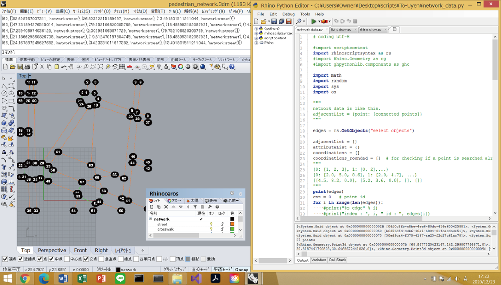
For those who are new to running Python in Rhinoceros, I would like to show you a screen transition.

First, start Rhinoceros and open the file of the modeled network. Then to the command

EditPythonScript

To start the editor. 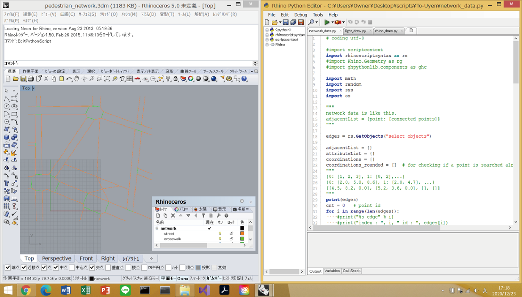In the figure above, the sidewalk (network \ street) and the pedestrian crossing (network \ crosswalk) are modeled separately in layers.

Click the green ▶ at the top of the editor to run the code. Then, in the command of Rhinoceros

select objects:

Will appear, select the entire network and press Enter.

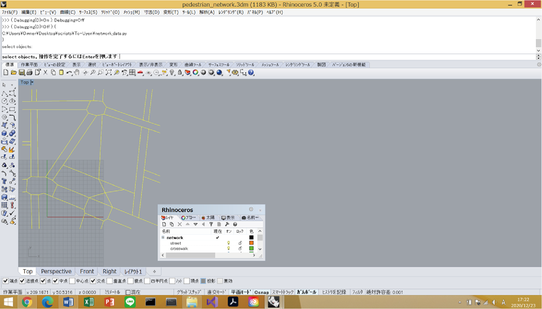
Then, advertisementList.txt, attributeList.txt, and coordinations.txt will be obtained, and the node positions will be numbered with text dots. Please use it as one of the means to check whether the completed data is correct.

[Next time] Read the exported network data in Python

As many of you may have noticed, in fact, in the code introduced in this article, we have already created the adjacent array itself once, and then exported it as .txt again, which is a roundabout thing. Python has a lot of modules related to network analysis, but I do this because it is often not available in Python on Rhinoceros.

Next time, I will retranslate the obtained .txt into an adjacent array to enable analysis on Python. → Read the network modeled by Rhinoceros in Python ③

The code related to the series of articles can be found below. → Related code

Homepage information

The contents of my research on architecture and urban planning mathematics and tips related to the research are available on my personal website. Eventually, I would like to create an analysis tool that can be used easily, so please come and take a look. → Shota Tabata's personal homepage

Load the network modeled with Rhinoceros in Python ②