EV3 x Python Machine Learning Part 2 Linear Regression

The content of this article is in beta and is subject to change. In this article, we will perform linear regression on line tracing using Educational version LEGO® MINDSTORMS EV3 (hereafter EV3) and Python environment. Please refer to the previous article for environment construction.

Machine learning with EV3 Part 1 Environment construction: here Machine learning with EV3 Part 2 Linear regression: This article Machine learning with EV3 Part 3 Classification: Coming soon

Environment in this article

• PC Windows10 Python 3.7.3 Development environment Visual Studio Code

• EV3 ev3dev

table of contents

1. What is linear regression?
2. What to do
3. EV3 model and driving course
4. Library to use and installation
5. Creating a program
6. IP settings for socket communication
7. Program execution
8. Execution result
9. Summary

What is linear regression?

Linear regression is an analytical method that finds the straight line that best fits a group of data when there is a distribution of data.

When there are two types of data groups as shown below, the results can be obtained by drawing a line that fits well with the data and making some predictions even for the data that you do not have. 　　　　　　　　

things to do

The main purpose is to perform linear regression with EV3, but it is necessary to connect the operation of EV3 with the inference by linear regression. This time, the goal is to perform line tracing with smooth running while performing linear regression according to the following procedure.

1. Get the value of the gyro sensor while running the elliptical course with a line trace
2. Draw the trajectory of the course from the two acquired values
3. Compare with the original course data and calculate the error for each lap to see how much the run was blurred.
4. Accumulate the error and turning value in csv data, perform linear regression based on the data, infer the turning value with less error, and feed it back.

EV3 model and driving course

The EV3 model used this time will be the following model. 　　　　 A color sensor is attached to the front of the car body, enabling line trace driving. A gyro sensor is attached to the rear part of the car body to acquire the angle at which the car body is facing. The traveling route is drawn using the value of this angle.

The elliptical course that runs this time uses the following course.

Library to use and installation

The libraries to be used additionally in addition to ev3dev this time are as follows.

• Numpy
• matplotlib
• Pandas
• Scikit-learn

Numpy
Numpy is a very popular library for doing numerical calculations in Python. You will be able to easily perform array calculation processing such as vector and matrix calculations. This time, it is used when storing the acquired sensor data in an array or performing calculations. Installation procedure

1. Launch a command prompt
2. Run the command pip install numpy

matplotlib matplotlib is a library often used when drawing graphs in Python. This time, it is used to draw the traveling route based on the gyro sensor data. Below the installation procedure

1. Launch a command prompt (It may be the one launched when installing Numpy)
2. Run the command pip install matplotlib

Pandas
Pandas is a library for handling data efficiently in Python. This time it is used to read the csv file. Below the installation procedure

1. Launch a command prompt (It may be the one launched when installing Numpy)
2. Run the command pip install pandas

sciki-learn scikit-learn is a Python machine learning library. Classification, regression, clustering, etc. can be implemented relatively easily. Below the installation procedure

1. Launch a command prompt (It may be the one launched when installing Numpy)
2. Run the command pip install scipy
3. Run the command pip install scikit-learn

Creating a program

This time, create the following three programs.

• EV3 side program data_get_gyro.py
• Comparison course data program course.py
• PC side program LinearRegression.py

Since there is a limit to the specifications of EV3, the configuration is such that numerical calculation and linear regression processing are performed on the PC side and the processing result value is sent to EV3. The relationship between each program is shown in the figure below.

EV3 side program

The EV3 side program is a program that is actually executed by EV3. Mainly, the EV3 will implement line tracing with a specified turning value, transfer of a gyro sensor using socket communication, and reception of feedback at a turning point.

Below, create the EV3 side program data_get_gyro.py in the workspace on VS Code. Please refer to Previous article for how to create a workspace and transfer the source code to EV3.

import time
import socket
import sys
from ev3dev2.button import Button
from ev3dev2.motor import LargeMotor, OUTPUT_B, OUTPUT_C
from ev3dev2.sensor import INPUT_2, INPUT_3
from ev3dev2.sensor.lego import GyroSensor, ColorSensor


 power range:-1050 -> 1050, turn_ratio range:-100 -> 100
def linetrace_steer(power, turn_ratio):
    global data_cycle
    if color.reflected_light_intensity > 30:
        ev3_motor_steer(power, turn_ratio*-1)
    else:
        ev3_motor_steer(power, turn_ratio)
    time.sleep(0.1)
    data_cycle += 1


def ev3_motor_steer(power, turn_ratio):
    if turn_ratio < 0:
        lm_b.run_forever(speed_sp=power*(1+turn_ratio/50))
        lm_c.run_forever(speed_sp=power)
    elif turn_ratio > 0:
        lm_b.run_forever(speed_sp=power)
        lm_c.run_forever(speed_sp=power*(1-turn_ratio/50))
    else:
        lm_b.run_forever(speed_sp=power)
        lm_c.run_forever(speed_sp=power)


def gyro_reset():
    time.sleep(1.0)
    gyro.mode = 'GYRO-ANG'
    gyro.mode = 'GYRO-RATE'
    gyro.mode = 'GYRO-ANG'
    time.sleep(1.0)


def dataget():
    global fb_steer     # feedback steering value
    global set_steer

    _gyro_data = gyro.value()  # gyro data
    _gyro_data_str = str(_gyro_data)
    s.send(_gyro_data_str.encode())
    print(_gyro_data_str)

    if ROUND_CHECK < _gyro_data:
        while not(button.up):
            ev3_motor_steer(0, 0)
            if fb_steer is None:
                fb_steer = s.recv(1024).decode()
                fb_steer_float = float(fb_steer)
                print(fb_steer_float)
                set_steer = set_steer - fb_steer_float
            if button.backspace:
                s.close
                print('End program')
                sys.exit()
        print('set_steer = ' + str(set_steer))
        # gyro reset
        gyro_reset()
        fb_steer = None


 sensors&motors definition
button = Button()
color = ColorSensor(INPUT_3)
gyro = GyroSensor(INPUT_2)
lm_b = LargeMotor(OUTPUT_B)
lm_c = LargeMotor(OUTPUT_C)

 gyro initialize
gyro_reset()

 variable initialize
data_cycle = 1           # counter
fb_steer = None    # Feedback turn
ROUND_CHECK = 355   # confirm one round

 motor initialize
lm_b.reset()
lm_c.reset()
set_power = 200
set_steer = 70

 get gyrodate and into array
with socket.socket(socket.AF_INET, socket.SOCK_STREAM) as s:
    s.connect(('169.254.207.161', 50010))    # your PC's Bluetooth IP & PORT
    while not(button.backspace):
        linetrace_steer(set_power, set_steer)
        if data_cycle % 4 == 0:    # gyro_get_frequency
            dataget()

lm_b.stop(stop_action='brake')
lm_c.stop(stop_action='brake')
print('End program')
sys.exit()

• Please note that if you comment out the EV3 environment in Japanese, an error will occur due to the nature of the character code. The s.connect (('169.254.207.161', 50010)) described in the latter half will be rewritten later according to the environment.

Comparison course data program

In the comparison course data program, data similar to the original course is generated for comparison with the ellipse of the locus drawn by the line trace. This program is not executed directly, but is created to be imported into LinearRegression.py, which will be created later. Create a folder called program on the desktop of the PC, create course.py as a text document in it, and describe the following contents.

import numpy as np
import matplotlib.pyplot as plt


def original_course(element_cnt, plot_interval):
    _element_cnt_f = element_cnt % 10    # element count fraction
    _element_cnt_unf = (element_cnt - _element_cnt_f)
    _element_cnt_s = _element_cnt_unf / 10  # element count one course section
    plot_interval = plot_interval + (_element_cnt_f*(plot_interval/_element_cnt_unf))

    _xcount = 1
    _ycount = 1
    _rcount = 1
    global P
    P = np.zeros(0)
    global Q
    Q = np.zeros(0)

    # 1
    while not _xcount > _element_cnt_s:
        _x1 = plot_interval * -1*_xcount
        _y1 = 0
        P = np.append(P, _x1)
        Q = np.append(Q, _y1)
        _xcount += 1

    # 2
    while not _xcount > _element_cnt_s * 2:
        _x2 = plot_interval * -1*_xcount
        _y2 = 0
        P = np.append(P, _x2)
        Q = np.append(Q, _y2)
        _xcount += 1

    # 3 cercle
    _rcount = 0
    while not _rcount > _element_cnt_s:
        _a1 = plot_interval*(_element_cnt_s*2) * -1    # cercle centerX
        _b1 = plot_interval*_element_cnt_s - plot_interval  # cercle centerY & radius
        _x3 = _a1 + _b1*np.cos(np.radians(270-(90 / _element_cnt_s*_rcount)))
        _y3 = _b1 + _b1*np.sin(np.radians(270-(90 / _element_cnt_s*_rcount)))
        P = np.append(P, _x3)
        Q = np.append(Q, _y3)
        _rcount += 1

    # 4
    while not _ycount > _element_cnt_s:
        _x4 = _x3
        _y4 = plot_interval*_ycount + _y3
        P = np.append(P, _x4)
        Q = np.append(Q, _y4)
        _ycount += 1

    # 5 cercle
    _rcount = 0
    while not _rcount > _element_cnt_s:
        _a2 = _a1    # cercle centerX
        _b2 = _y4    # cercle centerY
        _x5 = _a2 + _b1*np.cos(np.radians(180-(90 / _element_cnt_s*_rcount)))
        _y5 = _b2 + _b1*np.sin(np.radians(180-(90 / _element_cnt_s*_rcount)))
        P = np.append(P, _x5)
        Q = np.append(Q, _y5)
        _rcount += 1

    # 6
    _xcount = 1
    while not _xcount > _element_cnt_s:
        _x6 = _x5 + plot_interval*_xcount
        _y6 = _y5
        P = np.append(P, _x6)
        Q = np.append(Q, _y6)
        _xcount += 1

    # 7
    _xcount = 1
    while not _xcount > _element_cnt_s:
        _x7 = _x6 + plot_interval*_xcount
        _y7 = _y6
        P = np.append(P, _x7)
        Q = np.append(Q, _y7)
        _xcount += 1

    # 8 cercle
    _rcount = 0
    while not _rcount > _element_cnt_s:
        _a3 = 0     # cercle centerX
        _b3 = _y4    # cercle centerY
        _x8 = _a3 + _b1*np.cos(np.radians(90-(90 / _element_cnt_s*_rcount)))
        _y8 = _b3 + _b1*np.sin(np.radians(90-(90 / _element_cnt_s*_rcount)))
        P = np.append(P, _x8)
        Q = np.append(Q, _y8)
        _rcount += 1

    # 9
    _ycount = 1
    while not _ycount > _element_cnt_s:
        _x9 = _x8
        _y9 = plot_interval*_ycount*-1 + _y8
        P = np.append(P, _x9)
        Q = np.append(Q, _y9)
        _ycount += 1

    # 10 cercle
    _rcount = 0
    while not _rcount > _element_cnt_s:
        _a4 = 0     # cercle centerX
        _b4 = _b1     # cercle centerY
        _x10 = _a4 + _b1*np.cos(np.radians(0-(90 / _element_cnt_s*_rcount)))
        _y10 = _b4 + _b1*np.sin(np.radians(0-(90 / _element_cnt_s*_rcount)))
        P = np.append(P, _x10)
        Q = np.append(Q, _y10)
        _rcount += 1

if __name__ == '__main__':
    original_course(100, 30)
    plt.figure()
    plt.plot(P, Q, '-', color='blue')
    plt.show()

PC side program

The PC side program draws the travel route from the gyro sensor data sent from the EV3 and compares it with the original course data to calculate the error. In addition, the calculated error and turning value are recorded in a CSV file, and the appropriate turning value is fed back to EV3 as a result of inference by linear regression.

Create LinearRegression.py as a text document in the program folder in the same way as course.py, and describe the following contents.

import socket
import course   # course.py
import sys
import csv
import numpy as np
import matplotlib.pyplot as plt
import pandas as pd
import os.path
from sklearn import linear_model
clf = linear_model.LinearRegression()


 Feedback phase function
def feedback(element_cnt,
             plot_interval,
             min_steer,
             X,
             cur_steer,
             steers,
             errors):
    cnt = 1
    limit = 100

    # from course.py course coordinate point
    if not element_cnt == 1:
        course.original_course(element_cnt, plot_interval)

        _X_abs = np.abs(X)          # run coordinate point 'x'
        _P_abs = np.abs(course.P)   # from course.py course coordinate point 'x'
        _X_ave = _X_abs.mean()      # average
        _P_ave = _P_abs.mean()      # average
        _point_error = np.abs(_X_ave - _P_ave)    # point_average_error

        # add feedback_data to csv
        writedata = [cur_steer, _point_error]
        with open('datafile.csv', 'a', newline='') as f:
            writer = csv.writer(f)
 writer.writerow (writedata) # Write data

        steers = np.append(steers, cur_steer)  # append steer data
        errors = np.append(errors, _point_error)       # append error data
    print('steers = {}'.format(steers))
    print('errors = {}'.format(errors))
    print('len(errors) = {}'.format(len(errors)))

    if len(errors) > 1:
        if errors[-1] > errors[-2] and steers[-1] > min_steer:
            min_steer = steers[-1]
        errors = errors.reshape(-1, 1)

        clf.fit(errors, steers)    # linear regression

        while cnt < limit:
            ave_error = np.average(errors)
            input_error = cnt/(cnt+1) * ave_error
            input_error = input_error.reshape(-1, 1)
            predict_steer = clf.predict(input_error)
            if predict_steer > min_steer:
                break
            cnt += 1
        str_prd_steer = str(predict_steer[0])
        print('predict_steer = {}'.format(str_prd_steer))
        conn.send(str_prd_steer.encode())
        return predict_steer[0], min_steer, steers, errors
    else:
        cur_steer = cur_steer*2/3
        print('next_steer = {}'.format(cur_steer))
        conn.send(str(cur_steer).encode())
        return cur_steer, min_steer, steers, errors


 variable initialize
gyro = np.zeros(0)
element_cnt = 1   # element count
plot_interval = 30   # plot point interval
X = np.zeros(0)
Y = np.zeros(0)
steers = np.zeros(0)
errors = np.zeros(0)
Lap = 0
ROUND_CHECK = 355   # confirm one round
ini_steer = 70
cur_steer = ini_steer

 generate
if os.path.exists('datafile.csv') == False:
    writedata = ['steer', 'error']
 f = open ('datafile.csv','w', newline ='') # Open the file
    writer = csv.writer(f)
 writer.writerow (writedata) # Write data
    f.close()
 data = pd.read_csv ("datafile.csv", sep = ",") # read csv file
 steer_data = data.loc [:,'steer']. values # Set the swirl value in the objective variable (substitute the data in the steer column)
 error_data = data ['error'] .values # Set an error in the explanatory variable (substitute the data in the error column)
 min_steer = 0 # minimum value

for cnt, data in np.ndenumerate(steer_data):
    if error_data[cnt] < 900:
 steers = np.append (steers, data) # Substitute values other than course out
    elif data > min_steer:
 min_steer = data # update minimum
for data in error_data:
    if data < 900:
 errors = np.append (errors, data) # Substitute a value other than course out

 Main program
with socket.socket(socket.AF_INET, socket.SOCK_STREAM) as s:
    s.bind(('169.254.207.161', 50010))  # your PC's Bluetooth IP & PORT
    s.listen(1)
    print('Start program...')
    while True:
        conn, addr = s.accept()
        with conn:
            if len(errors) > 1:
                values = feedback(element_cnt,
                                  plot_interval,
                                  min_steer,
                                  X,
                                  cur_steer,
                                  steers,
                                  errors)
                cur_steer = values[0]
                min_steer = values[1]
                steers = values[2]
                errors = values[3]
            else:
                conn.send(str(cur_steer).encode())
            while True:
                gyro_data = conn.recv(1024).decode()
                if not gyro_data:
                    break
                gyro_data_float = float(gyro_data)  # change type
                gyro = np.append(gyro, gyro_data_float)    # gyro angle
                np.set_printoptions(suppress=True)

                cosgy = plot_interval * np.cos(np.radians(gyro)) * -1
                singy = plot_interval * np.sin(np.radians(gyro))
                X = np.append(X, np.sum(cosgy[0:element_cnt]))
                Y = np.append(Y, np.sum(singy[0:element_cnt]))

                if ROUND_CHECK < gyro_data_float:
                    plt.figure()
                    plt.plot(X, Y, '-', color='blue')
                    print('Plot file output')
                    print(str(Lap) + '-plot.png')
                    plt.savefig(str(Lap) + '-plot.png')
                    values = feedback(element_cnt,
                                      plot_interval,
                                      min_steer,
                                      X,
                                      cur_steer,
                                      steers,
                                      errors)
                    cur_steer = values[0]
                    min_steer = values[1]
                    steers = values[2]
                    errors = values[3]

                    # reset phase
                    element_cnt = 0
                    X = np.zeros(0)
                    Y = np.zeros(0)
                    gyro = []
                    plt.clf()   # figure clear
                    plot_interval = 30
                    Lap += 1

                element_cnt = element_cnt + 1   # Element count

 # Write to csv with an error of 1000 after going off course
            if element_cnt > 1:
                writedata = [cur_steer, 1000]
                f = open('datafile.csv', 'a', newline='')
                writer = csv.writer(f)
                writer.writerow(writedata)
                f.close()
            print('End program')
            sys.exit()

The s.bind (('169.254.207.161', 50010)) described in the latter half is changed by the following procedure according to the environment like the EV3 side program.

IP settings for socket communication

Data is exchanged between the EV3 side program and the PC side program via socket communication in order to give feedback on the value of the gyro sensor and the turning point, but the IP address described in the program is changed according to the environment. There is a need to.

Find out the IP address used for the Bluetooth connection between PC and EV3

When the PC and EV3 are connected via Bluetooth, the link local address of 169.254.XXX.YYY is assigned. Follow the steps below to find out the IP address.

1. Open a command prompt
2. Execute the ʻipconfig` command
3. Make a note of the IP address displayed in the displayed Ethernet Adapter Bluetooth Network Address.

data_get_gyro.py side setting

It is necessary to change the following description in the latter half of data_get_gyro.py.

    s.connect(('169.254.207.161', 50010))    # your PC's Bluetooth IP & PORT

The actual program editing is as follows.

After changing the description, transfer the workspace to EV3 on VS Code.

LinearRegression.py side setting

It is necessary to change the following description in the latter half of LinearRegression.py.

    s.bind(('169.254.207.161', 50010))  # your PC's Bluetooth IP & PORT

The actual editing of the program is as follows.

Program execution

After creating three programs and changing the description of the IP addresses in two places, execute the program. The following is the execution procedure.

1. Execute the command cd Desktop \ program from the command prompt (\ is synonymous with \ mark)
2. Execute the command python LinearRegression.py at the command prompt

• After execution, Start program ... is displayed and the system goes into a standby state. Allow access when the following pop-up appears.

3. Install EV3 at the start of the course

4. Open the SSH terminal of the EV3 connected on VS Code and execute cd ev3 workspace /

5. Run python3 data_get_gyro.py in the SSH terminal

6. Every lap the EV3 will stop near the starting point, so press the top button on the intelligent block to start the next lap.

• Repeat 6 thereafter

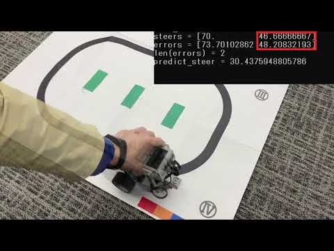
Execution result

After 6 laps, the result is as follows. The command prompt displays the turning value and error, the number of data (number of laps), and the next turning value for each lap. The value of the gyro sensor that is being sent to the program on the PC side is displayed on the SSH terminal on VS Code.

As for the operation, as shown in the following video, you can see that the line trace becomes smoother and the lap speed becomes faster with each lap.

When you open the CSV file that stores the data in Excel, the data is summarized as follows.

It is possible to graph it in the program, but this time I created a linear regression graph in Excel. It can be seen that the error at a certain turning value can be predicted to some extent.

Summary

This time, we performed a line trace and a linear regression to find the turning value from the traveling path. If you can get two related data, you can make a prediction in this way. It is a method that can be applied although it is necessary to consider what kind of data should be evaluated for the problem to be improved and customize it.

Next time, we will classify from the RGB numerical data acquired by the color sensor and judge several kinds of colors.