[GO] [Python3] Let's analyze data using machine learning! (Regression)
Target
--People who are interested in AI --People who are interested but don't know what to do --People who want to know what AI can do
Premise
--I have a Google account --Know the basic usage of Google Drive --Know the basic usage of Python3 --Does not deal with the theory of machine learning
See below for an overview of machine learning
Machine learning starting from scratch (overview of machine learning) --Qiita
goal
--You can predict the value of the target column of the table data with some accuracy. --Understand a few technical terms required for data analysis --Data can be displayed as a graph
Previous knowledge
The model used depends on the type of data to be predicted.
--Classification Predicting two types of labels, 0 or 1. Example) Positive / negative virus test, whether or not a customer cancels the service
--Regression Predicting numbers Example) Sales, number of visitors
This time we are dealing with regression
flow
- Preparing for Google Colaboratory
- initial screen --Runtime connection --Screen description --Add cell
- Read data
- Check the data --Top display (head) --Column description --Detailed information (describe) --Missing value and type confirmation (info) of each column --Histogram --Correlation confirmation (scatter_matrix) --Check the median house price by location (Basemap) --What you learned so far --part1
- Model training and prediction-part1 --Split data for learning / verification / testing ――Why do you prepare verification data? --Define a function to draw the accuracy of the prediction result --Linear regression learning and prediction accuracy visualization (no preprocessing) --XGBoost learning and prediction accuracy visualization (no preprocessing) --Random forest learning and visualization of prediction accuracy (no preprocessing) --What you learned so far --part2
- Pretreatment --Confirmation of outliers --Delete outliers --Split all_data into train and test
- Model training and prediction-part2 --Split data for learning / verification / testing
- Standardization --Learning of linear regression and visualization of prediction accuracy (with preprocessing) ---- XGBoost learning and visualization of prediction accuracy (with preprocessing) --Random forest learning and visualization of prediction accuracy (with preprocessing)
- Summary
- Other references
Preparing for Google Colaboratory
- Access Google Drive
- Create a folder for work (this time create a folder named handson)
- Move to the created folder
- Right-click => Other => Select Google Colaboratory
initial screen
It should look like the following (partially omitted)

Runtime connection
Open sample_data from the tab on the left and if you can confirm that california_housing_ {train/test} .csv exists, it's OK

Screen description
 red frame : text cell (markdown notation)
blue frame : code cell (python)
green frame : output result
red frame : text cell (markdown notation)
blue frame : code cell (python)
green frame : output result
You can execute a cell by pressing "Shift" + "Enter" or the start icon on the left side of the cell with the cell selected.
Execution is done cell by cell, and the value of the variable is retained even if the cell is moved.
The order in which the code cells are executed can be seen by the number on the left side of the blue frame .
Since the last variable of the code cell is output, there is no need to write print (hi) (super convenient!)
Add cell
You can add it with the "+ code", "+ text" on the upper left of the image below or the button displayed when you move the cursor to the center of the cell.

See below for detailed usage
-How to use Google Colab – Summary of advantages / disadvantages and basic operations of Google Colaboratory -How to use Google Colaboratory [Complete Manual] -Summary of how to use Google Colab --Qiita -Colaboratory Shortcut Memorandum --Qiita
From here, add cells as appropriate and execute
Data reading
This time, we will use the sample data california housing data. Sample data is prepared in advance in Colaboratory
import pandas as pd
pd.options.display.precision = 3

train = pd.read_csv('sample_data/california_housing_train.csv')
test = pd.read_csv('sample_data/california_housing_test.csv')
What is pandas? -wiki
pandas is a library that provides functions to support data analysis in the programming language Python. In particular, it provides data structures and operations for manipulating mathematical tables and time series data.
The number of digits after the decimal point is set in pd.options.display.precision (this time, for convenience of explanation, it is set to 3 digits after the decimal point).
You can read csv files with read_csv
Data confirmation
From here, let's look at the data
Top display (head)
train.head()
 You can check the table data up to the first 5 rows with
 head (if you enter a value in the argument, that number will be displayed)
Let's check test as well!
Description of each column
| Column name | Explanation |
|---|---|
| longitude | longitude |
| latitude | latitude |
| housing_median_age | Median age of blocks |
| total_rooms | Total number of rooms in the block |
| total_bedrooms | Total number of bedrooms in the block |
| population | Total number of people living in the block |
| households | Number of households per block |
| median_income | Median household income in a block[$ 10,000] |
| median_house_value | Median house prices in blocks[Dollar] |
Details of each column are as follows
The column to be predicted this time is median_house_value, which is called ** objective variable **.
The other columns are the data required for prediction and are called ** explanatory variables **.
Review detailed information (describe)
train.describe()

describe shows the following information for each column
| name | meaning |
|---|---|
| count | Number of lines |
| mean | Average value |
| std | standard deviation |
| min | minimum value |
| 25% | First quartile |
| 50% | Median |
| 75% | Third quartile |
| max | Maximum value |
Let's check test as well!
Missing value and type confirmation (info) of each column
train.info()
 Since the value of each item of
 Non-Null Count is 17000, which is the same as count confirmed in describe, it can be seen that there is no missing value.
If there is a missing value, it is necessary to complete it with some value or delete the line and do not use it for training data.
Let's check test as well!
Histogram
Installation of libraries required for graph display
import matplotlib.pyplot as plt
%matplotlib inline
Histogram display
train.hist(bins=50, figsize=(10, 10))

What is matplotlib? -wiki
Matplotlib is a graph drawing library for the programming language Python and its scientific computing library NumPy.
--% matplotlib inline is like magic
--Histogram display with hist
--bins is the number of bars
--Change the graph size with figsize (please choose if you like)
Let's check test as well!
Correlation confirmation (scatter_matrix)
pd.plotting.scatter_matrix(train, diagonal='kde', figsize=(10, 10))
 Select kernel density estimation with
 diagonal ='kde'
References
- pandas.plotting.scatter_matrix -About scatter_matrix-Qiita -Data visualization method by matplotlib (+ pandas) (5) --Qiita
Let's check test as well!
Check median home prices by location (Basemap)
Basemap installation
!apt-get install libgeos-3.5.0
!apt-get install libgeos-dev
!pip install https://github.com/matplotlib/basemap/archive/master.zip
When you see the following, restart the runtime from the button below
 After rebooting, run from above, including installing Basemap
OK when
After rebooting, run from above, including installing Basemap
OK when Successfully built base map is displayed
Install Basemap and define a function to display plots on the map
from mpl_toolkits.basemap import Basemap

def basemap(x, y, target):
  fig = plt.figure(dpi=300)
  xyrange = 0.5
  m = Basemap(projection="cyl", resolution="i", llcrnrlat=y.min()-xyrange, urcrnrlat=y.max()+xyrange, llcrnrlon=x.min()-xyrange, urcrnrlon=x.max()+xyrange)
  m.drawparallels(np.arange(-90, 90, 0.5), labels=[True, False, True, False],linewidth=0.0, fontsize=4)
  m.drawmeridians(np.arange(0, 360, 0.5), labels=[True, False, False, True],linewidth=0.0, rotation=45, fontsize=4)
  m.drawcoastlines(color='k')
  m.arcgisimage(service='World_Street_Map', verbose=True, xpixels=1000, dpi=300)
  plt.scatter(x, y, c=target, s=5, cmap=plt.get_cmap('jet'), alpha=0.4, linewidths=0)
  plt.colorbar()
Plot data around California
basemap(train['longitude'], train['latitude'], train['median_house_value'])
 References
-Visualize location information with Basemap-Qiita -How to install and use basemap on Google Colab?
Let's check test as well!
What I learned so far --part1
- The distribution of
trainandtestdata is almost the same (because each item and histogram of describe are almost similar) - The maximum values of
housing_median_ageandmedian_house_valueseem to be outliers (from the histogram). total_rooms,total_bedrooms,population, andhouseholdsare likely to be correlated (from the correlation graph).- Median home prices for seaside properties appear to be high (from Basemap)
What are outliers? -wiki
Outliers (outliers) are values that deviate significantly from other values in statistics.
Based on these, the next pretreatment should be performed However, in order to ** understand the importance of preprocessing **, we will work on learning machine learning models without dare to do it.
Model training and prediction-part1
Try learning without preprocessing The model used this time is as follows
--Linear regression (linear model) --XGBoost (decision tree model) --Random forest (decision tree model)
** Features of linear model **
--Features are numerical values --Cannot handle missing values --Standardization required ――The accuracy is not high by itself, and it is almost impossible to beat GBDT and neural networks.
** Features of decision tree model **
--Features are numerical values --Can handle missing values --Easy to get accuracy without parameter tuning ――The accuracy does not drop easily even if you add unnecessary features. --No need to scale (standardize or normalize) features
If you want to make predictions with a certain degree of accuracy, the decision tree model is easier and easier to handle. This time, as a comparison, we also deal with linear models. The linear model requires standardization of features, but in part1, we do not dare to standardize, and in part2 we check how much the accuracy changes.
What is standardization? -Data Science Handbook
Standardization in statistics is the operation of converting given data into data with a mean of 0 and a variance of 1.
Divide data for learning / verification / testing
from sklearn.model_selection import train_test_split
from sklearn.metrics import mean_squared_error

#Objective variable
obj_var = 'median_house_value'

#Explanatory variables for testing
x_test = test.drop(obj_var, axis=1)
#Objective variable for testing
y_test = test[obj_var]

#Explanatory variables for learning
x = train.drop(obj_var, axis=1)
#Objective variable for learning
y = train[obj_var]

#Divide the training data into training and verification
x_train, x_valid, y_train, y_valid = train_test_split(x, y, test_size=0.2, random_state=144, shuffle=True)
--Split data for training and verification with train_test_split
--Divided learning and verification at a ratio of 8: 2 with test_size = 0.2
--random_state is a pseudo-random number, otherwise the result will change each time it is executed.
Please use your favorite numbers
--Shuffle the split with shuffle = True
If not specified (False), 80% of the data is divided for learning and the remaining 20% is for verification.
--mean_squared_error will be used later to check the prediction accuracy
Why prepare verification data?
If the prediction accuracy is evaluated using only the training data and the test data, a model specialized for predicting the test data will be created (called overfitting).
For example, if you want to predict the weather using data from January to May of a certain year. If the prediction accuracy is improved only by evaluation using test data (overfitting), the weather from January to May of that year can be predicted well. However, the weather from January to May of the following year will be different from the previous year and the prediction accuracy will be worse. This is because it is unpredictable for unknown data.
If verification data is prepared so that the two data for verification and testing can be predicted with the same accuracy, it is possible to predict unknown data while maintaining a certain degree of accuracy (). Prevention of overfitting)
What is overfitting? --wiki
Overfitting (English: overfitting), overfitting (Kakigo) and overtraining (Kakushu, English: overtraining) are learned for training data in statistics and machine learning. However, it refers to a state in which unknown data (test data) cannot be adapted or generalized. Due to lack of generalization ability.
This time, we will use the simplest hold-out method. Besides, various such as cross validation and k-fold
Define a function to draw the accuracy of the prediction result
def predict_visualizer(valid, valid_predict, test, test_predict, title):
  valid_array = np.array(valid)
  test_array = np.array(test)
  va_pred_array = np.array(valid_predict)
  ts_pred_array = np.array(test_predict)
  y_values = np.concatenate([valid_array, va_pred_array]).flatten()
  ymin, ymax = np.amin(y_values), np.amax(y_values)
  fig = plt.figure(figsize=(10, 10))
  plt.scatter(valid_array, va_pred_array, label='valid', color='aqua', alpha=0.4)
  plt.scatter(test_array, ts_pred_array, label='test', color='tomato', alpha=0.4)
  plt.plot([ymin, ymax], [ymin, ymax])
  plt.xlabel('test', fontsize=24)
  plt.ylabel('predict', fontsize=24)
  plt.title(f'{title}-Test-Predict Plot', fontsize=24)
  plt.tick_params(labelsize=16)
  plt.legend()
  plt.show()
Linear regression learning and prediction accuracy visualization (no preprocessing)
from sklearn.linear_model import LinearRegression

lr = LinearRegression()
lr.fit(x_train, y_train)
y_pred = lr.predict(x_valid)
y_pred_test = lr.predict(x_test)
print('='*20)
print('LinearRegression')
print(f'valid_RMSE: {np.sqrt(mean_squared_error(y_valid, y_pred))}')
print(f'test_RMSE: {np.sqrt(mean_squared_error(y_test, y_pred_test))}')
predict_visualizer(y_valid, y_pred, y_test, y_pred_test, 'lr')

--Train the model with fit
--Predict the objective variable with predict
This time we predict two data for verification and two for testing respectively In order to evaluate the prediction accuracy, this time we use an average squared error called RMSE (Root Mean Squared Error). The calculation formula is as follows
$ N $: Total number of forecasted data $ y_i $: $ i $ th actual value $ \ hat {y_i} $: $ i $ th predicted value
Find the mean squared error with mean_sqared_error and take the square root with np.sqrt
From the result, RMSE was about 70,000.
When forecasting home prices with this model, it means that you can forecast with an average error of $ 70,000.
As a way of looking at the scatter plot, the closer the point is to the blue straight line, the more accurate the prediction.
Looking at this result, when test is 500000, it is not well predicted
This is thought to be due to the strong influence of outliers.
Let's look at other models in the same way
XGBoost learning and visualization of prediction results (no preprocessing)
import xgboost as XGB

xgb = XGB.XGBRegressor(random_state=144)
xgb.fit(x_train, y_train)
y_pred = xgb.predict(x_valid)
y_pred_test = xgb.predict(x_test)
print('='*20)
print('XGBRegressor')
print(f'valid_RMSE: {np.sqrt(mean_squared_error(y_valid, y_pred))}')
print(f'test_RMSE: {np.sqrt(mean_squared_error(y_test, y_pred_test))}')
predict_visualizer(y_valid, y_pred, y_test, y_pred_test, 'xgbr')
 From the result, RMSE was about 55,000.
It can be predicted with higher accuracy than the linear regression model.
However, it is the same that it is not well predicted when
From the result, RMSE was about 55,000.
It can be predicted with higher accuracy than the linear regression model.
However, it is the same that it is not well predicted when test is 500000.
Random forest training and visualization of prediction results (no preprocessing)
from sklearn.ensemble import RandomForestRegressor

rfr = RandomForestRegressor(random_state=144, n_estimators=100)
rfr.fit(x_train, y_train)
y_pred = rfr.predict(x_valid)
y_pred_test = rfr.predict(x_test)
print('='*20)
print('RandomForestClassifier')
print(f'valid_RMSE: {np.sqrt(mean_squared_error(y_valid, y_pred))}')
print(f'test_RMSE: {np.sqrt(mean_squared_error(y_test, y_pred_test))}')
predict_visualizer(y_valid, y_pred, y_test, y_pred_test, 'rfr')
 You can set the number of trees with
 n_estimators (100 this time)
From the result, RMSE was about 49,000.
Predicts with higher accuracy than XGBoost
However, it is the same that it is not well predicted when test is 500000.
What I learned so far-part2
| model | RMSE for verification | RMSE for testing |
|---|---|---|
| Linear regression | 70139 | 69766 |
| XGBoost | 55100 | 55100 |
| Random forest | 48458 | 49924 |
- Random forest makes the most accurate predictions
- None of the models are good at predicting when
testis 500000
It can be expected that the outliers seem to be bad, as mentioned in "What I learned so far-part 1". From here, pre-processing eliminates the effects of outliers.
Preprocessing
Combine all data (train and test) into one before preprocessing
train_mid = train.copy()
test_mid = test.copy()

train_mid['train_test'] = 'train'
test_mid['train_test'] = 'test'

all_data = pd.concat([train_mid, test_mid]).reset_index(drop=True)
all_data.head()
--Do not pollute the data of train and test with copy ()
--Added train_test column
--Combine multiple DataFrames with pd.concat
--Reset index with reset_index
--Delete the original index with drop = True (otherwise the original index will be included)
Check outliers
Item 2. of "What I learned so far --part 1".
The maximum value of
housing_median_ageandmedian_house_valueseems to be outliers (from the histogram)
To be specific
all_data['housing_median_age'].value_counts()
(Part of the result omitted)
 You can check the frequency of occurrence of each value with
 value_counts () in descending order.
From the results, it can be seen that the maximum value (see describe) of 52.0 is the highest.
Also check the median_house_value column
all_data['median_house_value'].value_counts()
(Part of the result omitted)
 From the results, it can be seen that the maximum value of 500001.0 is the highest.
From the two results, it was found that the maximum value of each was an outlier, which is considered to have an adverse effect on the prediction accuracy.
Remove outliers
Delete each maximum value
all_data = all_data.query(' housing_median_age < 52 and median_house_value < 500000 ').reset_index(drop=True)
Only rows that match the conditions can be extracted with query
Don't forget reset_index as the index will be skipped by extraction
Let's see how it changed with describe and hist!
- Test data should not be deleted in analysis competitions such as Kaggle and SIGNATE. In the case of analysis competition, only outliers of training data are deleted.
Split all_data into train and test
Since the pre-processing to delete the outliers is finished, split it into train and test
train = all_data.query(" train_test == 'train' ").drop('train_test', axis=1)
test = all_data.query(" train_test == 'test' ").drop('train_test', axis=1)
Model training and prediction-part2
Proceed in much the same way as "Model Learning and Prediction-part 1"
Divide data for learning / verification / testing
Same as the processing of part1
x_test = test.drop(obj_var, axis=1)
y_test = test[obj_var]

x = train.drop(obj_var, axis=1)
y = train[obj_var]

x_train, x_valid, y_train, y_valid = train_test_split(x, y, test_size=0.2, random_state=144, shuffle=True)
Standardization
Linear model requires standardization I didn't dare to do it in "Model Learning and Prediction-part 1"
from sklearn.preprocessing import StandardScaler

std_scl = StandardScaler()
x_train = std_scl.fit_transform(x_train)
x_valid = std_scl.transform(x_valid)
x_test = std_scl.transform(x_test)
Details of the StandardScalar method are below
Scale conversion (preprocessing) of data with Scikit-learn --Hatena Blog
Learning of linear regression and visualization of prediction accuracy (with preprocessing)
Same as the processing of part1
lr = LinearRegression()
lr.fit(x_train, y_train)
y_pred = lr.predict(x_valid)
y_pred_test = lr.predict(x_test)
print('='*20)
print('LinearRegression')
print(f'valid_RMSE: {np.sqrt(mean_squared_error(y_valid, y_pred))}')
print(f'test_RMSE: {np.sqrt(mean_squared_error(y_test, y_pred_test))}')
predict_visualizer(y_valid, y_pred, y_test, y_pred_test, 'lr')
 From the result, RMSE was about 60,000.
Since it was about 70,000 in part1, the accuracy has improved.
From the result, RMSE was about 60,000.
Since it was about 70,000 in part1, the accuracy has improved.
XGBoost learning and visualization of prediction accuracy (with preprocessing)
Same as the processing of part1
xgb = XGB.XGBRegressor(random_state=144)
xgb.fit(x_train, y_train)
y_pred = xgb.predict(x_valid)
y_pred_test = xgb.predict(x_test)
print('='*20)
print('XGBRegressor')
print(f'valid_RMSE: {np.sqrt(mean_squared_error(y_valid, y_pred))}')
print(f'test_RMSE: {np.sqrt(mean_squared_error(y_test, y_pred_test))}')
predict_visualizer(y_valid, y_pred, y_test, y_pred_test, 'xgbr')
 From the result, RMSE was about 50,000.
Since it was about 55,000 in part1, the accuracy has improved.
From the result, RMSE was about 50,000.
Since it was about 55,000 in part1, the accuracy has improved.
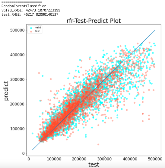
Random forest learning and prediction accuracy visualization (with preprocessing)
Same as the processing of part1
rfr = RandomForestRegressor(random_state=144, n_estimators=100)
rfr.fit(x_train, y_train)
y_pred = rfr.predict(x_valid)
y_pred_test = rfr.predict(x_test)
print('='*20)
print('RandomForestClassifier')
print(f'valid_RMSE: {np.sqrt(mean_squared_error(y_valid, y_pred))}')
print(f'test_RMSE: {np.sqrt(mean_squared_error(y_test, y_pred_test))}')
predict_visualizer(y_valid, y_pred, y_test, y_pred_test, 'rfr')
From the result, RMSE was about 45,000.
Since it was about 49,000 in part1, the accuracy has improved.
Summary
--I tried machine learning with Google Colaboratory
--Check the california_housing data
--Comparison of prediction accuracy with and without pretreatment
--It was confirmed that the prediction accuracy of the model learned by preprocessing was improved.
** part1 result **
| model | RMSE for verification | RMSE for testing |
|---|---|---|
| Linear regression | 70139 | 69766 |
| XGBoost | 55100 | 55100 |
| Random forest | 48458 | 49924 |
** part2 result **
| model | RMSE for verification | RMSE for testing |
|---|---|---|
| Linear regression | 58568 | 60750 |
| XGBoost | 48254 | 51184 |
| Random forest | 42473 | 45217 |
The only pre-processing we did this time was to delete outliers. However, data analysis, which is said to account for 80% of the total process of preprocessing, still has problems to be improved.
If you are interested in data analysis even a little, please try other preprocessing for better prediction accuracy.
Other references
-[1st California Home Price Forecast] Confirm accuracy without pretreatment -[2nd California Home Price Forecast] Feature Engineering & Data Cleaning (Data Cleansing) -[3rd California Home Price Forecast] Select and Evaluate the Best Machine Learning Model
Recommended Posts