Machine learning is often associated with deep learning, but there are many others. Also, it's not so deep because it's not good. So, let's try the data of previous article with another machine learning.

** Related series ** -Try to predict the exchange rate (FX) with the 1st TensorFlow (deep learning) ――Part 2 Try to predict the exchange rate (FX) by machine learning that is not deep -CNN edition of the 3rd TensorFlow (Deep Learning) Prediction of Forex (FX)

TL;DR 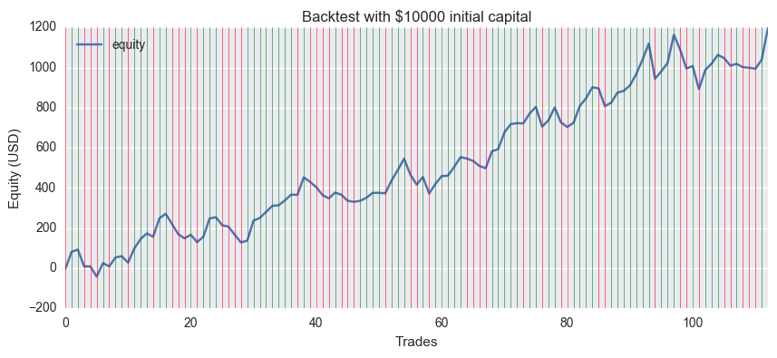I made a graph of the increase and decrease of assets. It's been 12% profit in about half a year, but it won't always work because the results aren't robust to the learning conditions.

** I have a Notebook on GitHub. ** ** Fork and play. https://github.com/hayatoy/ml-forex-prediction

Scikit-learn This is the first place to do machine learning with Python. If the installation is pip

pip install -U scikit-learn

I think it's okay.

Classifier selection

You can try them all, but I'm guessing that too linear will give good results for noisy data.

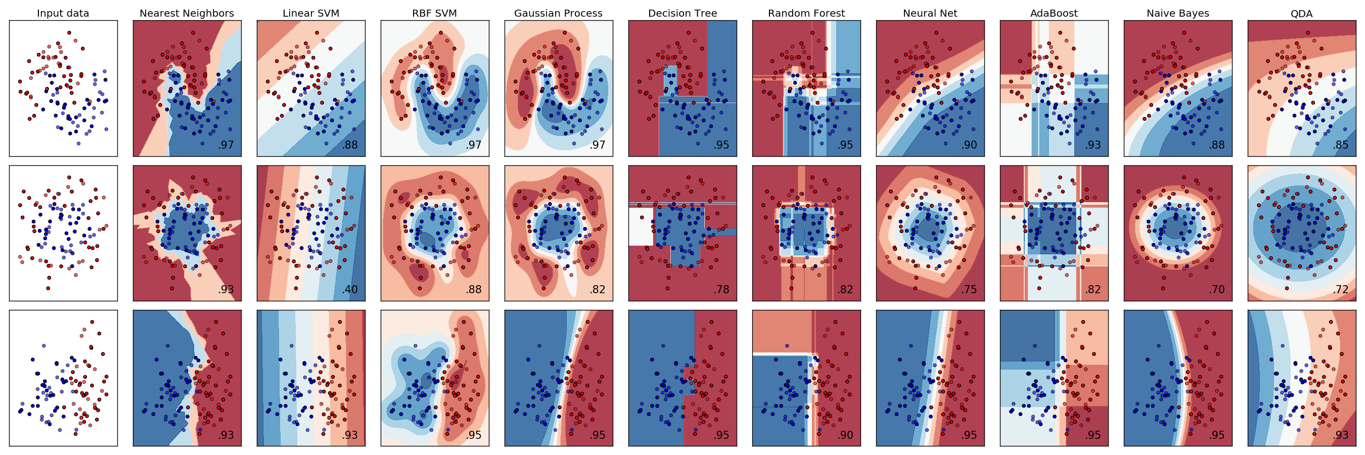An example of classification is like this [^ 1]. [^ 1]: Source: http://scikit-learn.org/stable/auto_examples/classification/plot_classifier_comparison.html

SVM (RBF), Naive Bayes area looks good.

Data processing

It seems that it will fit with the same shape, so I will use it as it is. When I thought about it, I got angry that the class was still 1 hot-vector. (Did you have any options?) It is a conversion from 1hot-vector to binary, but this time it is 2 classes, so it seems that you can just change the location to fetch.

>> train_y
[[ 0.  1.]
 [ 0.  1.]
 [ 1.  0.]
 [ 0.  1.]
 [ 0.  1.]
 [ 0.  1.]
 [ 1.  0.]
 [ 0.  1.]
 [ 1.  0.]
 [ 0.  1.]]
>> train_y[:,1]
[ 1.  1.  0.  1.  1.  1.  0.  1.  0.  1.]

This method cannot be used with multiple classes. I wonder if there is any cool way.

Let me learn

As before, 90% of the first half will be used for training and 10% for the second half will be used for testing. Below 0.502118 is worse than randomly predicting.

For the time being, implement with the default parameters fairly.

SVM (RBF)

from sklearn import svm
train_len = int(len(train_x)*0.9)
clf = svm.SVC(kernel='ref')
clf.fit(train_x[:train_len], train_y[:train_len,1])
clf.score(train_x[train_len:], train_y[train_len:,1])

Result: 0.49694435509810231

Gradient Boosting

from sklearn.ensemble import GradientBoostingClassifier
clf = GradientBoostingClassifier()
clf.fit(train_x[:train_len], train_y[:train_len,1])
clf.score(train_x[train_len:], train_y[train_len:,1])

Result: 0.52331939530395621

Random Forest

from sklearn.ensemble import RandomForestClassifier
clf = RandomForestClassifier(random_state=0)
clf.fit(train_x[:train_len], train_y[:train_len,1])
clf.score(train_x[train_len:], train_y[train_len:,1])

Result: 0.49726600192988096

Naive Bayes

from sklearn.naive_bayes import GaussianNB
clf = GaussianNB()
clf.fit(train_x[:train_len], train_y[:train_len,1])
clf.score(train_x[train_len:], train_y[train_len:,1])

Result: 0.50112576391122543

Nearest Neighbors

from sklearn.neighbors import KNeighborsClassifier
clf = KNeighborsClassifier()
clf.fit(train_x[:train_len], train_y[:train_len,1])
clf.score(train_x[train_len:], train_y[train_len:,1])

Result: 0.49726600192988096

QDA

from sklearn.discriminant_analysis import QuadraticDiscriminantAnalysis as QDA
clf = QDA()
clf.fit(train_x[:train_len], train_y[:train_len,1])
clf.score(train_x[train_len:], train_y[train_len:,1])

Result: 0.50981022836925061

Summary

Ranking	model	Accuracy
1	BiRNN(LSTM)	0.528883
2	Gradient Boosting	0.523319
3	QDA	0.509810
	Percentage of many classes	0.502118
4	Naive Bayes	0.501126
5	Random Forest	0.497266
6	Nearest Neighbors	0.497266
7	SVM (RBF)	0.496944

After all the last LSTM was the first place. Second place was Gradient Boosting, which is also popular in Kaggle. What is that? Is SVM the lowest, even though the parameters have not been adjusted? That should be ... I will try to search for the optimum parameters with Grid Search on another occasion.

Calculate PnL (Profit & Loss)

Just because the correct answer rate is bad does not mean that the profit and loss will be bad. Even with a correct answer rate of 50%, profit> loss is fine.

This data predicts whether the closing price for the next period will rise or fall. So (Next closing price-Current closing price) * Lot-Commission Was calculated as profit and loss. (Actually, it predicts when the current closing price is confirmed, so you can not take a position at the closing price. If it is the middle day of the week, it will only go up and down a little, but if you put the weekend in between, it will be a big value May be working)

github version of EUR / USD daily data. The green line means the correct answer and the red line means the wrong answer. The initial assets were $ 10,000, the trading unit was 10,000 currencies, the commission (spread) was 0, and the final profit was plus $ 1197. Even if you set the spread to an average of 2 pips, it is still about $ 900.

It looks good at first glance, but ... It seems that the model and data selection are not good, but just happened to fit nicely, as changing the training period quickly ruins it.

I have a notebook on GitHub, so give it a try. https://github.com/hayatoy/ml-forex-prediction

[PYTHON] Try to predict forex (FX) with non-deep machine learning

Classifier selection

Data processing

Let me learn

Summary

Calculate PnL (Profit & Loss)