[PYTHON] Newton's method for machine learning (from one variable to multiple variables)

An updated version of this article is available on my blog. See also here.

Introduction

In this article, I will review a little mathematically using Newton's method, referring to "Optimized mathematics that can be understood" [^ Kanatani] by Professor Kenichi Kanatani. At the same time, let's see how optimization using Python looks like this.

If you have any suggestions such as "This is better here", I would be grateful if you could give us guidance in the comments section.

1.1 For variables

For the sake of simplicity, let's start with the case of one variable. The value of the function $ f (x) $ around the point $ \ bar x $ on the $ x $ axis can be expanded by Taylor series.

It becomes. ($ ~ O (\ cdot) $ is Landau's O notation.) Here, if you ignore the terms of $ 3 $ and above,

It becomes. Consider maximizing this. The following equation can be obtained by differentiating with $ \ Delta x $ and setting it as $ 0 $.

Where $ f ^ {\ prime} (\ bar x) = \ cfrac {df} {dx} (\ bar x), ~~ f ^ {\ prime \ prime} (\ bar x) = \ cfrac {d If you set ^ 2f} {dx ^ 2} (\ bar x) $ and solve for $ \ Delta x $,

It becomes. Here, since $ \ Delta x = x-\ bar x $,

can be obtained. The quadratic approximation of $ f (x) $ (approximation by a quadratic function) is performed to find the value of $ x $ that gives the extremum of the quadratic function. It is the meaning of calculation. Next, a quadratic approximation is performed around the value of $ x $ that gives this extremum, and a value that becomes an extremum is searched for. The idea of Newton's method is to gradually approach the extremum of $ f (x) $ by repeating this.

In summary, the procedure is as follows.

** Newton's method (1) **

1. Give the initial value of $ x $
2. Update as $ \ bar x \ leftarrow x $ as follows. $ x \leftarrow \bar x - \cfrac{f^{\prime}(\bar x)}{f^{\prime\prime}(\bar x)} $ 3. ~|~x - \bar x~| \leq \delta~Check if it is. If false, return to step 2. If true, returns x.

1.1 Example

Let's try Newton's method with an analytically solvable and simple example in the reference book. Consider the following function $ f $.

The first-order and second-order derivatives of this are

is. Now consider a quadratic approximation.

$ \ Delta x = x-\ bar x $, so

It becomes. Now let's plot the quadratic approximation around $ f $ and its $ \ bar x = 2 $ on the same plane!

f = lambda x: x**3 - 2*x**2 + x + 3
d1f = lambda x: 3*x**2 - 4*x + 1
d2f = lambda x: 6*x - 4
f2 = lambda bar_x, x: f(bar_x) + d1f(bar_x)*(x - bar_x) + d2f(bar_x)*(x - bar_x)**2

x = np.linspace(-10, 10, num=100)
plt.plot(x, f(x), label="original")
plt.plot(x, f2(2, x), label="2nd order approximation")
plt.legend()
plt.xlim((-10, 10))

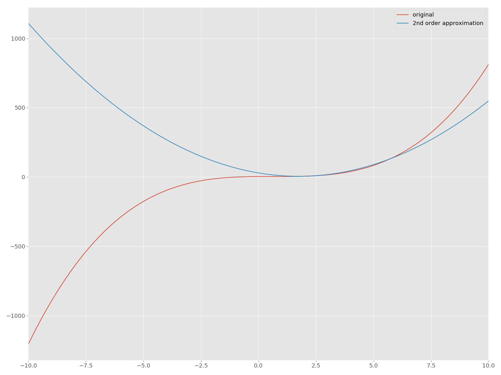
The red curve is the original function $ f $, and the blue quadratic function is the approximated curve. Now, let's implement Newton's method in Python and find a solution that gives a stop point. In this article, we will not dare to use useful APIs such as scipy.optimize.

newton_1v.py

class Newton(object):
    def __init__(self, f, d1f, d2f, f2):
        self.f = f
        self.d1f = d1f
        self.d2f = d2f
        self.f2 = f2

    def _update(self, bar_x):
        d1f = self.d1f
        d2f = self.d2f
        return bar_x - d1f(bar_x)/d2f(bar_x)

    def solve(self, init_x, n_iter, tol):
        bar_x = init_x
        for i in range(n_iter):
            x = self._update(bar_x)
            error = abs(x - bar_x)
            print("|Δx| = {0:.2f}, x = {1:.2f}".format(error, x))
            bar_x = x
            if error < tol:
                break
        return x

def _main():
    f = lambda x: x**3 - 2*x**2 + x + 3
    d1f = lambda x: 3*x**2 - 4*x + 1
    d2f = lambda x: 6*x - 4
    f2 = lambda bar_x, x: f(bar_x) + d1f(bar_x)*(x - bar_x) + d2f(bar_x)*(x - bar_x)**2

    newton = Newton(f=f, d1f=d1f, d2f=d2f, f2=f2)
    res = newton.solve(init_x=10, n_iter=100, tol=0.01)
    print("Solution is {0:.2f}".format(res))

if __name__ == "__main__":
    _main()

If you do this, you will get the following output:

|Δx| = 4.66, x = 5.34
|Δx| = 2.32, x = 3.01
|Δx| = 1.15, x = 1.86
|Δx| = 0.55, x = 1.31
|Δx| = 0.24, x = 1.08
|Δx| = 0.07, x = 1.01
|Δx| = 0.01, x = 1.00
Solution is 1.00

The plot looks like this: It is monotonically decreasing toward 0. In fact, the solution obtained is 1.00, which is consistent with the analytical solution of $ 1.00 $. You can also get $ 1/3 $ by changing the initial value. For example, if ʻinit_xis-10, the numerical solution will be 0.33`. However, if the opposite is returned, it also means that the solution obtained depends on the initial value.

The code up to this point has been uploaded to Gist, so please see here for details.

2. For multiple variables

Next, let's consider the case of multiple variables. Function $ f at the point $ [\ bar x_1, ~ \ cdots, ~ \ bar x_n] $ near the point $ [\ bar x_1 + \ Delta x_1, ~ \ cdots, ~ \ bar x_n + \ Delta x_n] $ (\ bar x_1, ~ \ cdots, ~ \ bar x_n) When the value of $ is expanded by Taylor, $ f(\bar x_1 + \Delta x_1,~\cdots,~\bar x_n + \Delta x_n) = \bar f + \sum^{n}_{i=1} \frac{\partial \bar f}{\partial x\_{i}}\Delta x\_i + \frac{1}{2!} \sum^{n}\_{i,~j=1} \frac{\partial^2 \bar f}{\partial x\_i\partial x\_j}\Delta x\_i \Delta x\_j + \cdots $

It becomes. I will not derive this development because it is out of the scope of this article, but I think it would be good to refer to the lecture by Professor Saburo Higuchi [^ Taylor] because it is very easy to understand.

Now, let's return to the Taylor expansion. The $ \ bar f $ used in the Taylor expansion earlier is the value of the function $ f $ at the point $ [\ bar x_1, ~ \ cdots, ~ \ bar x_n] $. As with the one variable, ignore the third and subsequent terms and set $ 0 $ after differentiating with $ \ Delta x_i $.

This is also the case for other variables, so considering the Hessian matrix [^ Hessian]

is. $ \ Nabla $ is a symbol called nabla. For example, taking a two-variable scalar function as an example, a vector having a first-order partial differential equation is created as shown below. This is called a gradient.

Comparing with Eq. (1), you can see that the gradient vector corresponds to the first-order derivative and the Hessian matrix corresponds to the second-order derivative. Let's solve this for $ \ boldsymbol {x} $, paying attention to $ \ Delta \ boldsymbol {x} = \ boldsymbol {x}-\ boldsymbol {\ bar x} $.

From the above, the Newton method at this time has the following procedure.

** Newton's method (2) **

1. Give the initial value of $ \ boldsymbol {x} $
2. Calculate the values of the gradient $ \ nabla f $ and the Hessian matrix $ \ boldsymbol {H} $ at $ \ boldsymbol {\ bar x} $.
3. Calculate the solution of the following linear equation. $ \boldsymbol{H}\Delta\boldsymbol{x} = - \nabla f $
4. Updated $ \ boldsymbol {x} . $ \boldsymbol{x}\leftarrow \boldsymbol{x} + \Delta \boldsymbol{x} $$
5. ||\Delta\boldsymbol{x}|| \leq \deltaIf\boldsymbol{x}return it. If false, return to Step2.

2.1 Example

Now, consider the following function, which is also covered in the reference book [^ Kanatani].

A quadratic approximation of this around $ \ boldsymbol {\ bar x} = [\ bar x_0, \ bar x_1] $ is

And the gradient $ \ nabla f $ and the Hessian matrix $ \ boldsymbol {H} $ are

It becomes. Let's implement it in Python.

newton_mult.py

import numpy as np
import matplotlib.pyplot as plt

plt.style.use("ggplot")
plt.rcParams["font.size"] = 13
plt.rcParams["figure.figsize"] = 16, 12

class MultiNewton(object):
    def __init__(self, f, dx0_f, dx1_f, grad_f, hesse):
        self.f = f
        self.dx0_f = dx0_f
        self.dx1_f = dx1_f
        self.grad_f = grad_f
        self.hesse = hesse

    def _compute_dx(self, bar_x):
        grad = self.grad_f(bar_x)
        hesse = self.hesse(bar_x)
        dx = np.linalg.solve(hesse, -grad)
        return dx

    def solve(self, init_x, n_iter=100, tol=0.01, step_width=1.0):
        self.hist = np.zeros(n_iter)
        bar_x = init_x
        for i in range(n_iter):
            dx = self._compute_dx(bar_x)
            # update
            x = bar_x + dx*step_width
            print("x = [{0:.2f} {1:.2f}]".format(x[0], x[1]))

            bar_x = x
            norm_dx = np.linalg.norm(dx)
            self.hist[i] += norm_dx
            if norm_dx < tol:
                self.hist = self.hist[:i]
                break
        return x

def _main():
    f = lambda x: x[0]**3 + x[1]**3 - 9*x[0]*x[1] + 27
    dx0_f = lambda x: 3*x[0]**2 - 9*x[1]
    dx1_f = lambda x: 3*x[1]**2 - 9*x[0]
    grad_f = lambda x: np.array([dx0_f(x), dx1_f(x)])
    hesse = lambda x: np.array([[6*x[0], -9],[-9, 6*x[1]]])

    init_x = np.array([10, 8])
    solver = MultiNewton(f, dx0_f, dx1_f, grad_f, hesse)
    res = solver.solve(init_x=init_x, n_iter=100, step_width=1.0)
    print("Solution is x = [{0:.2f} {1:.2f}]".format(res[0], res[1]))

    errors = solver.hist
    epochs = np.arange(0, errors.shape[0])

    plt.plot(epochs, errors)
    plt.tight_layout()
    plt.savefig('error_mult.png')

if __name__ == "__main__":
    _main()

If you do this, you will get the following output: The solution is $ [3, 3] $ and one of the analytical solutions can be obtained.

x = [5.76 5.08]
x = [3.84 3.67]
x = [3.14 3.12]
x = [3.01 3.00]
x = [3.00 3.00]
Solution is x = [3.00 3.00]

Finally, how will it converge?||\Delta x||It ends with a graph of the transition of.

in conclusion

So far, we have outlined Newton's method in the case of multiple variables, although the example starts with one variable and is two variables. When studying machine learning algorithms, you will often find parameters that define some reference value and give the minimum (or maximum) value of the function. At this time, you use an optimization method such as Newton's method. A quick glance at the mathematical formulas may seem difficult, but if you read it from scratch, you will find that if you have knowledge of university mathematics, you can follow it unexpectedly.

In recent years, you can try machine learning algorithms immediately by using scikit-learn etc., but it is also important to understand what is inside. That is the end of this article.

(If you feel like it, write the quasi-Newton method, etc.)

References [^ Kanatani]: Kenichi Kanatani, "From the basic principles of optimized mathematics to the calculation method," Kyoritsu Shuppan. [^ Taylor]: Calculus / Exercise (2006) L09 Taylor expansion of multivariable functions (9.1) Derivation | Youtube [^ Hessian]: Extremum of multivariable functions and Hessian matrix | Beautiful story of high school mathematics