[PYTHON] Linear regression with statsmodels

I used to use scipy.stats.linregress as a linear regression in Python, but I introduced statsmodels because it has few functions and is difficult to use. I've only used it for 2 hours, so I may have misunderstood something fundamentally. I've only used it for 2 hours, so I'm sorry.

The following describes how to use OLS (ordinary least square) of statsmodels. Click here for official materials http://statsmodels.sourceforge.net/stable/regression.html

Installation

Normally with pip.

$ sudo pip install statsmodels

The code below also uses numpy and matplotlib, so install them if you don't have them.

$ sudo pip install numpy
$ sudo pip install matplotlib

Simple example

For the time being, as the simplest example

y = a + bx + \varepsilon

Consider linear regression in the model. In other words, given the data of $ (x_i, y_i) $, the parameter $ (a, b) $ is determined so that the error $ \ sum \ varepsilon_i ^ 2 $ is minimized.

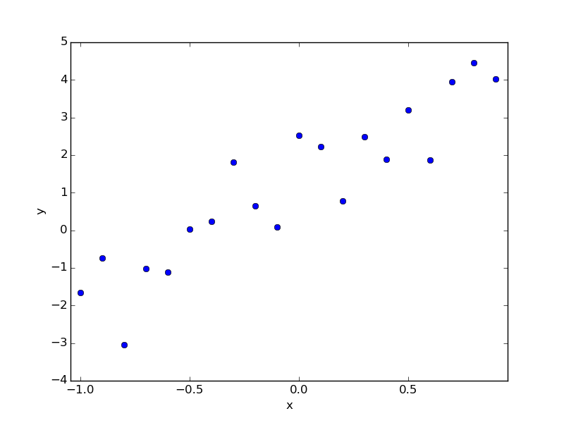
For example, suppose you have the following data. This is the data I made now, and if I answered first, it would be a = 1.0, b = 3.0, but I pretend I don't know and find it by regression.

data.txt

#      x        y
  -1.000   -1.656
  -0.900   -0.734
  -0.800   -3.036
  -0.700   -1.026
  -0.600   -1.104
  -0.500    0.023
  -0.400    0.246
  -0.300    1.817
  -0.200    0.651
  -0.100    0.082
  -0.000    2.524
   0.100    2.231
   0.200    0.783
   0.300    2.489
   0.400    1.892
   0.500    3.207
   0.600    1.868
   0.700    3.954
   0.800    4.447
   0.900    4.024

The regression for this is as follows.

regression.py

# coding: utf-8
import numpy as np
import statsmodels.api as sm
import matplotlib.pyplot as plt

#Read data
data = np.loadtxt("data.txt")
x = data.T[0]
y = data.T[1]

#Number of samples
nsample = x.size

#Magic(Commentary later)
X = np.column_stack((np.repeat(1, nsample), x))

#Regression execution
model = sm.OLS(y, X)
results = model.fit()

#View result summary
print results.summary()

#Get parameter estimates
a, b = results.params

#Show plot
plt.plot(x, y, 'o')
plt.plot(x, a+b*x)
plt.text(0, 0, "a={:8.3f}, b={:8.3f}".format(a,b))
plt.show()

When executed, the following text and graph will be displayed.

                            OLS Regression Results                            
==============================================================================
Dep. Variable:                      y   R-squared:                       0.831
Model:                            OLS   Adj. R-squared:                  0.822
Method:                 Least Squares   F-statistic:                     88.59
Date:                Thu, 25 Dec 2014   Prob (F-statistic):           2.25e-08
Time:                        14:07:16   Log-Likelihood:                -24.450
No. Observations:                  20   AIC:                             52.90
Df Residuals:                      18   BIC:                             54.89
Df Model:                           1                                         
Covariance Type:            nonrobust                                         
==============================================================================
                 coef    std err          t      P>|t|      [95.0% Conf. Int.]
------------------------------------------------------------------------------
const          1.2922      0.194      6.647      0.000         0.884     1.701
x1             3.1611      0.336      9.412      0.000         2.455     3.867
==============================================================================
Omnibus:                        0.801   Durbin-Watson:                   2.495
Prob(Omnibus):                  0.670   Jarque-Bera (JB):                0.653
Skew:                          -0.402   Prob(JB):                        0.721
Kurtosis:                       2.628   Cond. No.                         1.74
==============================================================================

Warnings:
[1] Standard Errors assume that the covariance matrix of the errors is correctly specified.

It will be like this.

Linear basis function model

In the model mentioned above, the relationship between x and y was a linear expression, but in life we often want to consider a more complicated relationship between x and y. Therefore, by using a linear basis function model, it becomes possible to express a relatively diverse relationship between x and y.

y = \beta_0 + \beta_1 \phi_1(x) + \beta_2\phi_2(x) + \cdots + \beta_{M-1}\phi_{M-1}(x) + \varepsilon

Here, $ x and y $ are data, $ \ phi_j (x) $ is a known function, and $ \ beta_j $ is a parameter to be obtained. Note that this formula can be easily set to $ \ phi_0 (x) \ equiv 1 $.

y = \sum_{j=0}^{M-1} \beta_j\phi_j(x) + \varepsilon

Can also be written. For example, if $ M = 3, \ phi_1 (x) = x, \ phi_2 (x) = x ^ 2 $, then the quadratic function $ y = \ beta_0 + \ beta_1x + \ beta_2x ^ 2 + \ varepsilon $ ..

When performing regression with statsmodels, you need to enter the data $ (x_i, y_i) $ and the information of the known function $ \ phi_j (x) $, but it is awkward to insert the function information directly, so $ Enter the following matrix that summarizes the information of x_i $ and $ \ phi_j (x_i) $. (When M = 3)

X = \begin{Bmatrix}
\phi_0(x_0) & \phi_1(x_0) & \phi_2(x_0) \\
\phi_0(x_1) & \phi_1(x_1) & \phi_2(x_1) \\
\phi_0(x_2) & \phi_1(x_2) & \phi_2(x_2) \\
& \vdots & \\
\end{Bmatrix}

Here, $ \ phi_0 (x) \ equiv 1 $, so the first column of this matrix is all 1. That's why I added the column `` `np.repeat (1, nsample) ``` in the previous code as "magic".

So, if we change the way this matrix X is created, linear regression of any model is possible.

Somewhat complicated example

As an example

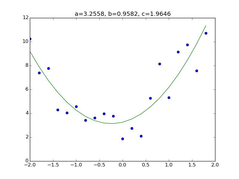
y = a + bx + cx^2 + \varepsilon

Consider the model. All you have to do is add a column corresponding to $ x ^ 2 $ to the matrix X part of the previous code. First, prepare the data set. As usual, the answer is a = 3.0, b = 1.0, c = 2.0.

data.txt

#      x        y
  -2.000   10.260
  -1.800    7.403
  -1.600    7.779
  -1.400    4.310
  -1.200    4.051
  -1.000    4.577
  -0.800    3.416
  -0.600    3.628
  -0.400    3.968
  -0.200    3.780
  -0.000    1.873
   0.200    2.741
   0.400    2.106
   0.600    5.286
   0.800    8.138
   1.000    5.316
   1.200    9.159
   1.400    9.748
   1.600    7.585
   1.800   10.726

The code is below. However, I changed only the part where the matrix X was created and the number of the last parameters.

regression_2.py

# coding: utf-8
import numpy as np
import statsmodels.api as sm
import matplotlib.pyplot as plt

#Data read
data = np.loadtxt("data.txt")
x = data.T[0]
y = data.T[1]

#Number of samples
nsample = x.size

#Creating matrix X
X = np.column_stack((np.repeat(1, nsample), x, x**2))

#Perform regression
model = sm.OLS(y, X)
results = model.fit()

#View result summary
print results.summary()

#Get parameter estimates
a, b, c = results.params

#Display as a graph
plt.plot(x, y, 'o')
plt.plot(x, a+b*x+c*x**2)
plt.title("a={:.4f}, b={:.4f}, c={:.4f}".format(a,b,c))
plt.show()

Other

In addition to OLS (ordinary least squares), statsmodels also has WLS (weighted least squares), so write it if you like.