[PYTHON] Plate reproduction of Bayesian linear regression (PRML §3.3)

greeting

I'm @naoya_t, the secretary of Machine Learning Advent Calendar 2013, which started today. I look forward to working with you again this year. (The day has changed in Japan time. I'm sorry it was so late. I was just in time for Argentine Standard Time (GMT-3)!)

The content of this Advent calendar article can be anything related to data science, such as pattern recognition, machine learning, natural language processing, and data mining. The amount does not matter as long as it follows the theme. (Summary of read parts of PRML, MLaPP, etc., implementation, dissertation introduction, mathematical expansion, etc.)

Let's enjoy both the writers and the readers!

Today's topic

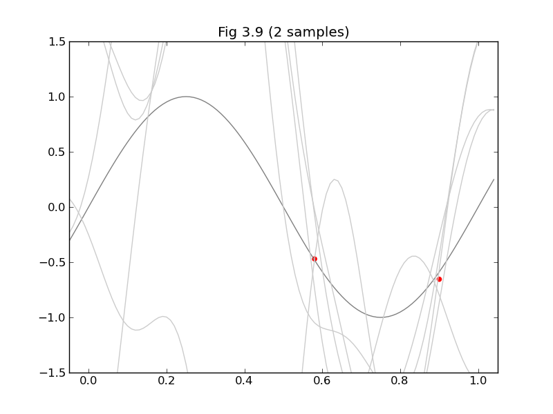
Today, since it is a light topic from PRML that everyone loves, I would like to reproduce Figure 3.8 and Figure 3.9 from "Bayesian Linear Regression" in §3.3.

図3.8 図3.9

I was thinking of drawing a 3D graph of the equivalent kernel (Fig. 3.10), but the time was up. (I will add it when I feel like it!)

Required calculations

Since the caption in Figure 3.8 says, "The model consists of nine Gaussian (basis) functions of the form (3.4)". Gaussian basis set $ \ phi_j (x) = exp \ left (-\ frac {(x- \ mu_j) ^ 2} {2s ^ 2} \ right) $ as appropriate within the range of x = [0,1]( I'll try arranging 9 pieces (or evenly).

Figure 3.8 is the predicted distributionp(t|\mathbf{x},\mathbf{t},\alpha,\beta)=N(t|\mathbf{m}_N\mathbf{\phi(x)},\sigma_N^2(\mathbf{x})) (3.58)You can draw if you can get the mean and variance of. Needed for this $ \ mathbf {m} _N $, $ \ mathbf {S} _N $, $ \ sigma_N ^ 2 (\ mathbf {x}) $

\mathbf{S}_N^{-1}=\alpha I+\beta\Phi^\mathrm{T}\Phi (3.54)
\mathbf{m}_N=\beta\mathbf{S}_N\Phi^\mathrm{T}\mathbf{t} (3.53)
\sigma_N^2(\mathbf{x})=\frac1\beta+\mathbf{\phi(x)}^\mathrm{T}\mathbf{S}_N\mathbf{\phi(x)} (3.59)

It can be found by. The $ \ Phi $ that appears here is the design matrix (3.16) that everyone is familiar with. Assemble from the basis function $ \ phi_j (x) $ and the input data $ \ mathbf {x} $.

Figure 3.9 is\mathbf{w}Posterior distribution ofp(\mathbf{w}|\mathbf{t})=N(\mathbf{w}|\mathbf{m}_N,\mathbf{S}_N) (3.49)From\mathbf{w}Sampling 5 each, about eachy(x,\mathbf{w})=\mathbf{w}^\mathrm{T}\mathbf{\phi(x)}Just plot.

code

`fig38_39.py`


#!/usr/bin/env python
# -*- coding: utf-8 -*-

from pylab import *

S     = 0.1
ALPHA = 0.1
BETA  = 9

def sub(xs, ts):
    # φj(x)Adopts Gaussian basis functions
    def gaussian_basis_func(s, mu):
        return lambda x:exp(-(x - mu)**2 / (2 * s**2))

    # φ(x)
    def gaussian_basis_funcs(s, xs):
        return [gaussian_basis_func(s, mu) for mu in xs]

    xs9 = arange(0, 1.01, 0.125) # 9 points
    bases = gaussian_basis_funcs(S, xs9)

    N = size(xs) #Data score
    M = size(bases) #Number of basis functions

    def Phi(x):
        return array([basis(x) for basis in bases])

    # Design matrix
    PHI = array(map(Phi, xs))
    PHI.resize(N, M)

    # predictive distribution
    def predictive_dist_func(alpha, beta):
        S_N_inv = alpha * eye(M) + beta * dot(PHI.T, PHI)
        m_N = beta * solve(S_N_inv, dot(PHI.T, ts)) # 20.1

        def func(x):
            Phi_x = Phi(x)
            mu = dot(m_N.T, Phi_x)
            s2_N = 1.0/beta + dot(Phi_x.T, solve(S_N_inv, Phi_x))
            return (mu, s2_N)

        return m_N, S_N_inv, func

    xmin = -0.05
    xmax =  1.05
    ymin = -1.5
    ymax =  1.5

    #
    #Figure 3.8
    #
    clf()
    axis([xmin, xmax, ymin, ymax])
    title("Fig 3.8 (%d sample%s)" % (N, 's' if N > 1 else ''))

    x_ = arange(xmin, xmax, 0.01)
    plot(x_, sin(x_*pi*2), color='gray')

    m_N, S_N_inv, f = predictive_dist_func(ALPHA, BETA)

    y_h = []
    y_m = []
    y_l = []
    for mu, s2 in map(f, x_):
        s = sqrt(s2)
        y_m.append(mu)
        y_h.append(mu + s)
        y_l.append(mu - s)

    fill_between(x_, y_h, y_l, color='#cccccc')
    plot(x_, y_m, color='#000000')

    scatter(xs, ts, color='r', marker='o')
    show()

    #
    #Figure 3.9
    #
    clf()
    axis([xmin, xmax, ymin, ymax])
    title("Fig 3.9 (%d sample%s)" % (N, 's' if N > 1 else ''))

    x_ = arange(xmin, xmax, 0.01)
    plot(x_, sin(x_*pi*2), color='gray')

    for i in range(5):
        w = multivariate_normal(m_N, inv(S_N_inv), 1).T
        y = lambda x: dot(w.T, Phi(x))[0]
        plot(x_, y(x_), color='#cccccc')

    scatter(xs, ts, color='r', marker='o')
    show()


def main():
    #Sample data (adds Gaussian noise)
    xs = arange(0, 1.01, 0.02)
    ts = sin(xs*pi*2) + normal(loc=0.0, scale=0.1, size=size(xs))

    #Pick up an appropriate number from the sample data
    def randidx(n, k):
        r = range(n)
        shuffle(r)
        return sort(r[0:k])

    for k in (1, 2, 5, 20):
        indices = randidx(size(xs), k)
        sub(xs[indices], ts[indices])


if __name__ == '__main__':
    main()

did it!

At the end

Last year, it was pointed out that I skipped too much from the first day, so it is not because of the writing time, but this year I am sorry that I could not meet everyone's expectations with a slightly lighter theme setting.

The person in charge of 12/2 is @ puriketu99. stay tuned!