Outline of method

The overall flow is shown in Fig. 1 described in the paper.

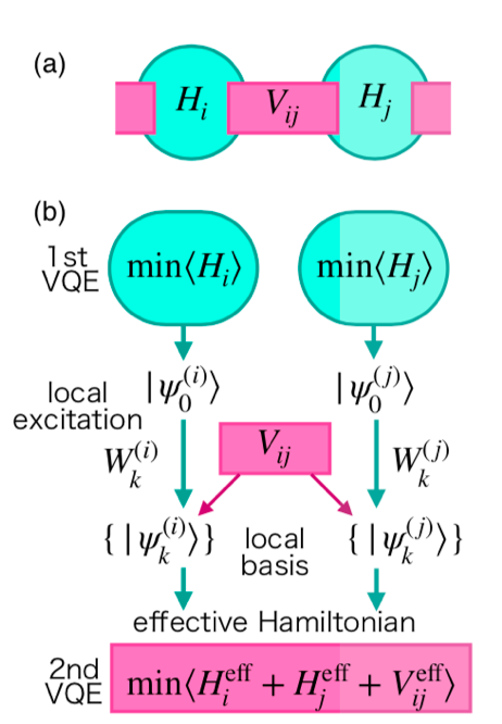
1. Decompose Hamiltonian into interactions with partial systems. (a)
2. Calculate the ground state by calculating the partial system with VQE. (b, 1st VQE)
3. Create a local basis from the interaction and ground state. (local basis)
4. Compute the Hamiltonian matrix elements using the local basis.
5. Create an effective Hamiltonian that incorporates interactions. (effective Hamiltonian)
6. Perform a VQE on a valid Hamiltonian. (2nd VQE)

I understand that it is possible to reduce the number of qubits used in the stage of making the number of local bases correspond to qubits. If you create a local basis with 3, but the number is $ K $, the number of qubits required to express this is $ \ lceil \ log_2 {K} \ rceil $. From this, the number of qubits required to represent the valid Hamiltonian created in 5 is $ 2 \ lceil \ log_2 {K} \ rceil $ because the two subsystems are combined.

Consider the case where two 4-qubit Heisenberg models calculated in the paper are connected. If you try to calculate without decomposition, you will need 8 qubits. When decomposed and calculated, VQE is initially performed using 4 qubits, and since the number of interactions is $ K = 7 $, 3 qubits are required for each subsystem in the next calculation. Since two of these subsystems are united, the total number of qubits required is six. Since it is a toy model, it is a small amount, but you can see that it has been reduced to $ 8 \ to 6 $.

Next, we will look at how to create a local basis and an effective Hamiltonian.

Details of the method

Hamiltonian definition

Divide the Hamiltonian into subsystems and interactions.

$ \ mathcal {H} \ i $ represents the Hamiltonian of the partial system, and $ V {ij} $ represents the interaction acting on the partial systems $ i $ and $ j $. Here, $ V \ _ {ij} $ assumes the following form.

$ W ^ {(i)} \ _ {k} $ represents the operator that works on the subsystem $ i $, and $ W ^ {(j)} \ _ {k} $ represents the operator that works on the subsystem $ j $. ..

Creating a local basis

First, find the ground state of $ \ mathcal {H} \ _i $ using VQE. The variational quantum circuit used in VQE is expressed as $ U_i (\ theta ^ {(i)}) $, and the obtained ground state is expressed as $ \ ket {\ psi ^ {(i)} _0} . ( i $ corresponds to the index of the partial system $ i $.) $ \ theta ^ {(i), *} $ is an optimized parameter

Then, $ \ ket {\ psi ^ {(i)} _0} $ is

Can be expressed as. Create a local basis from $ W ^ {(i)} \ _ {k} $ included in the interaction with this $ \ ket {\ psi ^ {(i)} _ 0} . ( k $ corresponds to the type of interaction operator.)

Using this local basis, we will calculate the effective Hamiltonian by rewriting the original Hamiltonian. Only $ W ^ {(i)} _1 $ is defined as an identity operator, and if there are $ K $ interaction operators, a total of $ K + 1 $ local rules are created. I will. (Hereafter, the number of local bases is represented by $ K $.) At this stage, it is not necessarily $ \ brakett {\ psi ^ {(i)} \ _ k} {\ psi ^ {(i)} \ _ l} = \ delta \ _ {kl} $. This is orthonormalized using Gram-Schmidt's orthonormalization method. The orthonormalized local basis is represented as $ \ ket {\ tilde {\ psi} ^ {(i)} \ _k} $.

$ C_k $ is a normalization constant to satisfy $ \ brakett {\ tilde {\ psi} ^ {(i)} \ _k} {\ tilde {\ psi} ^ {(i)} \ _k} = 1 $ Become.

If you write this out concretely, $ k = 1 $ remains as it is

\begin{align}
\ket{\tilde{\psi}^{(i)}_1} &= \frac{1}{C_1} \ket{\psi^{(i)}_1} \\
C_1 &= \sqrt{\brakett{\psi^{(i)}_1}{\psi^{(i)}_1}}
\end{align}

It will be. At $ k = 2 $

\begin{align}
\ket{\tilde{\psi}^{(i)}_2} &= \frac{1}{C_2}\biggl(\ket{\psi^{(i)}_2} - \brakett{\tilde{\psi}^{(i)}_1}{\psi^{(i)}_2} \ket{\tilde{\psi}^{(i)}_1}\biggr) \\
&= \frac{1}{C_2}\biggl(\ket{\psi^{(i)}_2} - \frac{1}{C_1^2}\brakett{\psi^{(i)}_1}{\psi^{(i)}_2} \ket{\psi^{(i)}_1}\biggr)
\end{align}

The same calculation can be done after $ k> 2 $. To find $ \ ket {\ tilde {\ psi} ^ {(i)} \ _k} $ from this, the inner product of the local basis $ \ brakett {\ psi ^ {(i)} _1} {\ psi ^ {(i) You can see that we need to calculate)} _2} $. Inner product

\begin{align}
\brakett{\psi^{(i)}_k}{\psi^{(i)}_l} = \braket{\psi^{(i)}_0}{W^{(i)\dagger}_{k}W^{(i)}_{l}}{\psi^{(i)}_0}
\end{align}

Since it can be expanded with $ \ ket {\ psi ^ {(i)} \ _0} $, $ W ^ {(i) \ dagger} \ _ {k} W ^ {(i)} \ _ {l} $ You can see that you can measure the expected value. (The process of taking the expected value with $ \ ket {\ psi ^ {(i)} \ _0} $ will appear in later calculations.) Note that, for example, $ W ^ {(i) \ dagger} = X ^ {(i)} \ _0, W ^ {(i)} \ _ {l} = Y ^ {(i)} \ _0 $ If $ W ^ {(i) \ dagger} \ _ {k} W ^ {(i)} \ _ {l} = X ^ {(i)} \ _ 0Y ^ {(i)} \ _ 0 = iZ ^ The point is that you need to measure the expected value of $ Z ^ {(i)} \ _0 $ after converting it to an observable using the relationship between {(i)} \ _0 $ and the Pauli operator. (The value obtained by multiplying this measurement by $ i $ is the value of the matrix element.)

$ \ Ket {\ tilde {\ psi} ^ {(i)} \ _k} $ for ease of later calculations $ \ ket {\ psi ^ {(i)} \ _ {k ^ {\ The coefficient when expanded with prime}}} $ is defined as $ P \ _ {kk ^ {\ prime}} $ and expressed as follows.

\begin{align}
\ket{\tilde{\psi}^{(i)}_k} &= \sum^K_{k^{\prime}=1}P^{(i)}_{kk^{\prime}} \ket{\psi^{(i)}_{k^{\prime}}} \\
\end{align}

You can create a matrix $ P $ by measuring $ \ brakett {\ psi ^ {(i)} \ _ k} {\ psi ^ {(i)} \ _l} $ respectively.

This orthonormalized local basis is hereafter simply referred to as the local basis.

Creating a valid Hamiltonian

Calculate the matrix elements of $ \ mathcal {H} \ _ i, V \ _ {ij} $ using $ \ ket {\ tilde {\ psi} ^ {(i)} _k} $.

Partial effective Hamiltonian

First of all, the valid Hamiltonian matrix element $ (\ mathcal {H} ^ {\ text {eff}} \ _i) \ _ {kl} $ of $ \ mathcal {H} \ _i $ is

\begin{align}
    (\mathcal{H}^{\text{eff}}_i)_{kl} &= \braket{\tilde{\psi}^{(i)}_k }{\mathcal{H}_i}{\tilde{\psi}^{(i)}_l} \\
    &= \sum_{k^{\prime},l^{\prime}} \braket{\psi^{(i)}_{k^{\prime}} }{P^{(i)*}_{kk^{\prime}} \mathcal{H}_i P^{(i)}_{ll^{\prime}}}{ \psi^{(i)}_{l^{\prime}}} \\
    &= \sum_{k^{\prime},l^{\prime}} P^{(i)*}_{kk^{\prime}} \braket{\psi^{(i)}_0}{ W^{(i)}_{k^{\prime}}\;^{\dagger}\mathcal{H}_i W^{(i)}_{l^{\prime}}}{ \psi^{(i)}_0}  P^{(i)}_{ll^{\prime}} \\
&= \biggl(P^{(i)*} \bar{\mathcal{H}}^{\text{eff}}_i P^{(i)T} \biggr)_{kl}
\end{align}

It will be. Where $ \ bar {\ mathcal {H}} ^ {\ text {eff}} \ _i $ is

\begin{align}
 (\bar{\mathcal{H}}^{\text{eff}}_i)_{kl} &= \braket{\psi^{(i)}_k }{\mathcal{H}_i}{ \psi^{(i)}_l} \\
    &= \braket{\psi^{(i)}_0}{ W^{(i)}_{k}\;^{\dagger}\mathcal{H}_i W^{(i)}_{l}}{ \psi^{(i)}_0}
\end{align}

It is a matrix element defined by. To create a matrix element for $ \ mathcal {H} ^ {\ text {eff}} \ _i $, use $ \ ket {\ psi ^ {(i)} _0} $

\begin{align}
W^{(i)}_{k}\;^{\dagger}\mathcal{H}_i W^{(i)}_{l}
\end{align}

You need to measure the expected value of $ \ bar {\ mathcal {H}} ^ {\ text {eff}} \ _i $ to find the matrix element. By using this and the matrix $ P $ used when creating the local basis, you can create $ \ mathcal {H} ^ {\ text {eff}} \ _i $.

Effective interaction Hamiltonian

Interaction at the local basis

\begin{align}
V_{ij} = \sum_{k} v_{k} W^{(i)}_{k} W^{(j)}_{k}
\end{align}

The matrix elements are calculated by sandwiching from both sides. Since $ W ^ {(i)} \ _ {k} and W ^ {(j)} \ _ {k} $ act on the partial systems $ i $ and $ j $, respectively.

\begin{align}
(V^{\text{eff}}_{ij})_{kk^{\prime}ll^{\prime}} &= \bra{\tilde{\psi}^{(i)}_k} \bra{\tilde{\psi}^{(j)}_{k^{\prime}}} V_{ij} \ket{\tilde{\psi}^{(i)}_l} \ket{\tilde{\psi}^{(j)}_{l^{\prime}}} \\
&= \sum_{\nu} v_{\nu} \braket{\tilde{\psi}^{(i)}_k }{W^{(i)}_{\nu}}{ \tilde{\psi}^{(i)}_l} \braket{\tilde{\psi}^{(j)}_{k^{\prime}} }{W^{(j)}_{\nu}}{ \tilde{\psi}^{(j)}_{l^{\prime}}}
\end{align}

Then, $ \ braket {\ tilde {\ psi} ^ {(i)} \ _ k} {W ^ {(i)} \ _ {\ nu}} {\ tilde {\ psi} ^ {(i)} \ You need to find _l} $. If you develop this in the same way as before

\begin{align}
\braket{\tilde{\psi}^{(i)}_{k}}{W^{(i)}_{\nu}}{\tilde{\psi}^{(i)}_l} &= \sum_{k^{\prime},l^{\prime}} P^{(i)*}_{kk^{\prime}}  \braket{\psi^{(i)}_0}{ W^{(i)}_{k^{\prime}}\;^{\dagger}W^{(i)}_{\nu} W^{(i)}_{l^{\prime}}}{ \psi^{(i)}_0} P^{(i)}_{ll^{\prime}} \\
&= \biggl(P^{(i)*} \bar{W}^{(i), \text{eff}}_{\nu} P^{(i)T} \biggr)_{kl}
\end{align}

And here

\begin{align}
(\bar{W}^{(i), \text{eff}}_{\nu})_{kl} &\equiv \braket{\psi^{(i)}_k}{ W^{(i)}_{\nu}}{\psi^{(i)}_l} = \braket{\psi^{(i)}_0 }{ W^{(i)}_{k}\;^{\dagger}W^{(i)}_{\nu} W^{(i)}_{l}}{ \psi^{(i)}_0}
\end{align}

Is defined as. From the above, to calculate $ V ^ {\ text {eff}} \ _ {ij} $, use $ \ ket {\ psi ^ {(i)} _0} $

\begin{align}
W^{(i)}_{k}\;^{\dagger}W^{(i)}_{\nu} W^{(i)}_{l}
\end{align}

Observe the expected value of $ (\ bar {W} ^ {(i), \ text {eff}} \ _ {\ nu}) and calculate the matrix element of $. You can create $ V ^ {\ text {eff}} \ _ {ij} $ by using this and the matrix $ P $ used to create the local basis.

Represented by a gate

So far we have found the effective Hamiltonian matrix elements. The ground state can be obtained from the eigenvalues and eigenstates by diagonalizing the $ K ^ 2 \ times K ^ 2 $ dimensional matrix obtained by integrating the two subsystems represented by the local basis without using a quantum computer. I think that it is necessary to represent it with the gate corresponding to the matrix element in order to calculate using a quantum computer.

For $ (\ mathcal {H} ^ {\ text {eff}} \ _i) _ {kl} $, the corresponding Hamiltonian operator is

\begin{align}
(\mathcal{H}^{\text{eff}}_i)_{kl}\ket{\tilde{\psi}^{(i)}_k} \bra{\tilde{\psi}^{(i)}_l}
\end{align}

Will be. This $ \ ket {\ tilde {\ psi} ^ {(i)} \ _ k} \ bra {\ tilde {\ psi} ^ {(i)} \ _l} $ must be represented by a gate. Before that, we first need to associate the local basis $ \ ket {\ tilde {\ psi} ^ {(i)} \ _k} $ with the qubit. For example, if $ K = 7 $, you should consider the following correspondence.

\begin{align}
    \ket{\tilde{\psi}^{(i)}_1} &= \ket{000} \\ 
    \ket{\tilde{\psi}^{(i)}_2} &= \ket{001} \\ 
    \ket{\tilde{\psi}^{(i)}_3} &= \ket{010} \\ 
    \ket{\tilde{\psi}^{(i)}_4} &= \ket{011} \\ 
    \ket{\tilde{\psi}^{(i)}_5} &= \ket{100} \\ 
    \ket{\tilde{\psi}^{(i)}_6} &= \ket{101} \\ 
    \ket{\tilde{\psi}^{(i)}_7} &= \ket{110}
\end{align}

From this correspondence, for example

\begin{align}
\ket{\tilde{\psi}^{(i)}_1}\bra{\tilde{\psi}^{(i)}_2} &= \ket{000}\bra{001}\\
&= \ket{0}\bra{0}_0 \otimes \ket{0}\bra{0}_1 \otimes \ket{0}\bra{1}_2
\end{align}

Therefore, after that, the projection operator $ \ ket {0} \ bra {0} \ _0 $ of each qubit can be represented by using a gate. Focusing on one qubit

\begin{align}
Z &= \ket{0}\bra{0} - \ket{1}\bra{1} \\
I &= \ket{0}\bra{0} + \ket{1}\bra{1}
\end{align}

From $ \ ket {0} \ bra {0}, \ ket {1} \ bra {1} $ can be expressed using $ Z, I $. In the same way

\begin{align}
\ket{0}\bra{0} &= \frac{1}{2}(I + Z) \\
\ket{1}\bra{1} &= \frac{1}{2}(I - Z) \\
\ket{0}\bra{1} &= \frac{1}{2}(I + iY) \\
\ket{1}\bra{0} &= \frac{1}{2}(I - iY)
\end{align}

I think it can be converted using. Since Hamiltonian is Hermitian, I think it can be expanded using these gates and real coefficients.

Effective Hamiltonian

Find the ground state with VQE using the valid Hamiltonian of $ \ mathcal {H} \ _ {i}, \ mathcal {H} \ _ {j}, V \ _ {ij} $ found above as a new subsystem. ..

\begin{align}
\mathcal{H}^{\text{eff}}_{ij} = \mathcal{H}^{\text{eff}}_i + \mathcal{H}^{\text{eff}}_j + V^{\text{eff}}_{ij}
\end{align}

If there are only two subsystems, the above process needs to be executed only once, but if there are three or more, it is necessary to repeat the process according to the division.

Qubit number

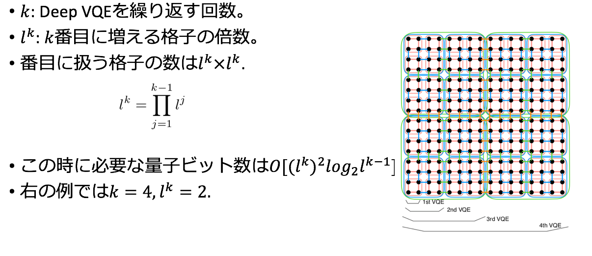
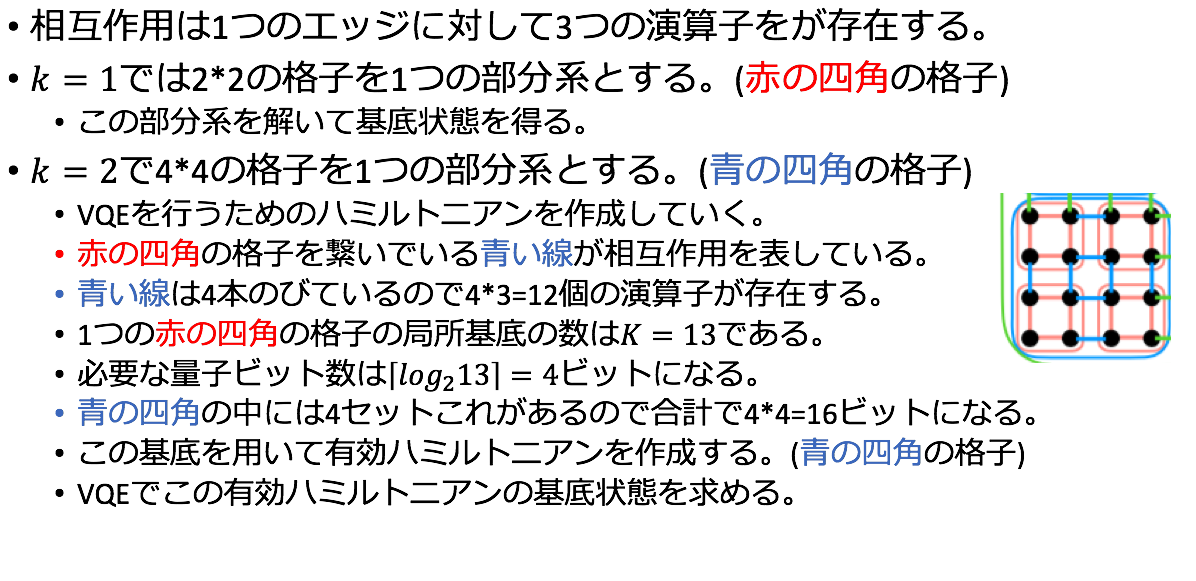
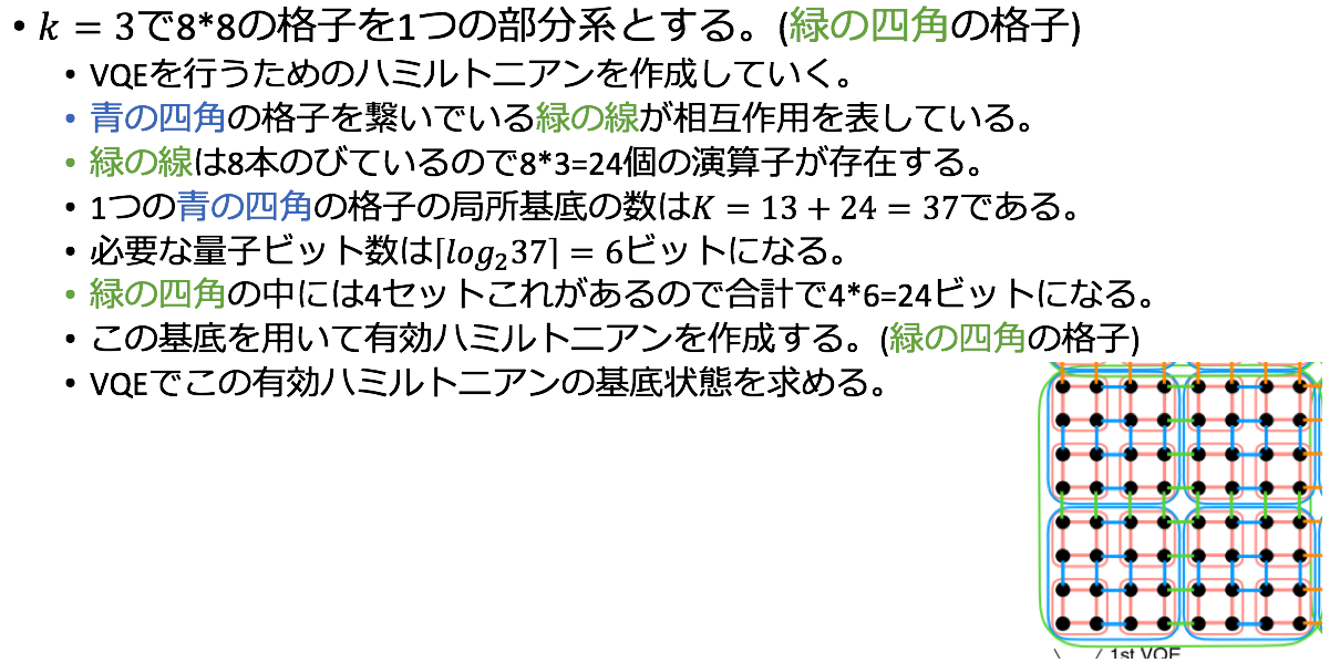
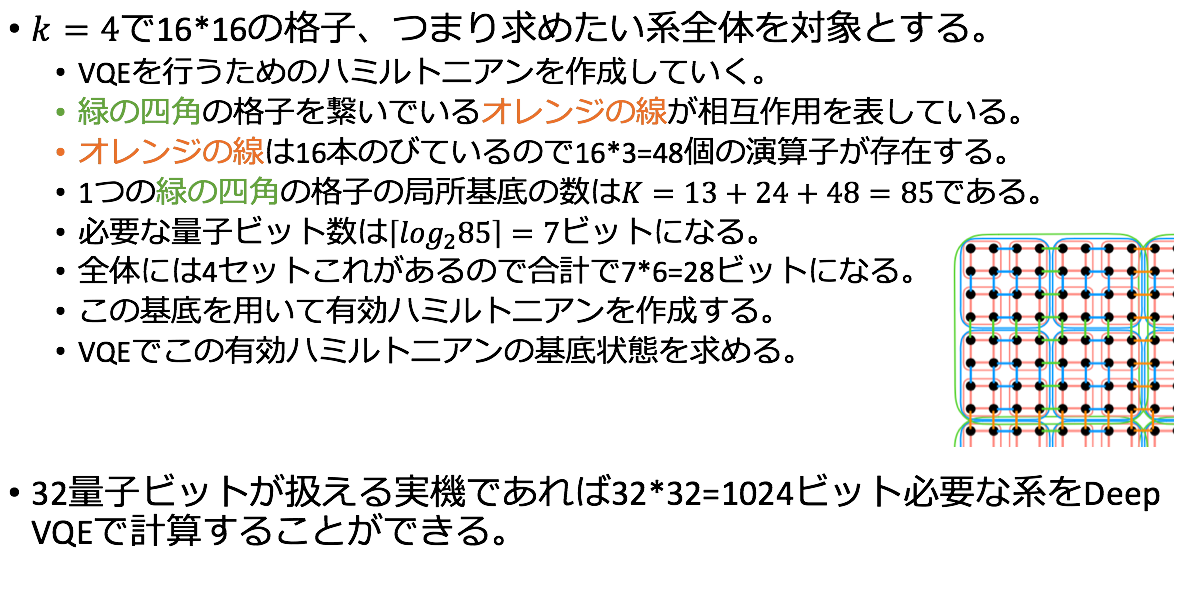
If the number of the first subsystem is $ N $ and the number of qubits required for one subsystem is $ n $, if you try to solve it at once without dividing the entire system, the total number of qubits is $ M = nN $ quantum. You will need a bit. On the other hand, when the division is large, if the number of local bases is $ K $, the required number of qubits is $ m = N \ lceil \ log \ _2 {K} \ rceil $, which is $ M \ to m $. It has been reduced.

In the paper, the required number of bits is specifically discussed using a model in which a partial system of 4 qubits is repeated two-dimensionally. I summarized the calculation method of the number of qubits required for the image below.

Calculation result

Introducing the calculation results calculated in the paper.

Model a

First, as shown in the figure below, it is a model in which a partial system composed of 4 qubits is connected in a one-dimensional manner. (In the implementation part, I calculated a model in which these two are connected.)

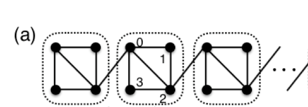
The subsystem consists of the following antiferromagnetic Heisenberg model.

\begin{align}
    \mathcal{H}_i &= \sum_{E=(\mu, \nu)}(X^{(i)}_{\mu}X^{(i)}_{\nu} + Y^{(i)}_{\mu}Y^{(i)}_{\nu} + Z^{(i)}_{\mu}Z^{(i)}_{\nu}) \\
    &= \sum_{E=(\mu, \nu)}\sum_{A=X,y,Z}A^{(i)}_{\mu} A^{(i)}_{\nu} 
\end{align}

Here the edges are $ E = \ {(0,1), (1,2), (2,3), (3,0), (0,2) } $. The following interactions work between the subsystems.

\begin{align}
    V_{ij} = \sum_{A=X,Y,Z}(A^{(i)}_{0} A^{(j)}_{2} + A^{(i)}_{2} A^{(j)}_{0})
\end{align}

The calculation results are summarized in the table below.

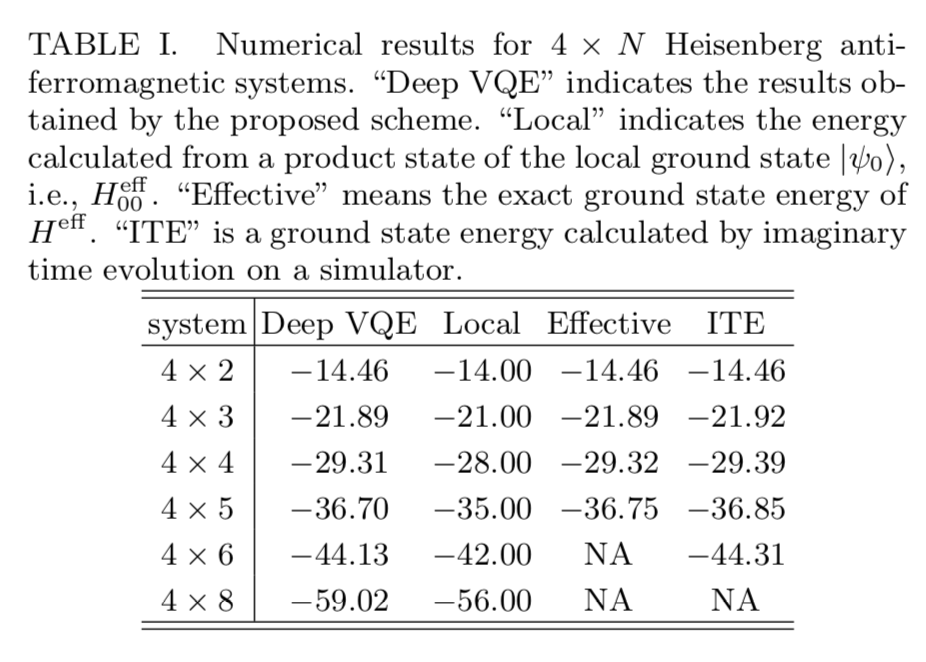
The total energy of the partial system where Local ignores the interaction, Effective is the energy obtained by diagonalizing the Hamiltonian, ITE represents each energy obtained by the imaginary time evolution method.

Effective and ITE are not listed because the size increases at $ N = 8 $. $ N = 2 $ matches the values of Deep VQE, Effective, and ITE. When $ N> 2 $, the effective and deep VQE values for ITE become slightly larger and deviate, but you can see that they give a good approximation. It can be seen that an approximate energy value can be obtained by using Deep VQE even for systems that cannot be calculated directly by ITE.

Model b

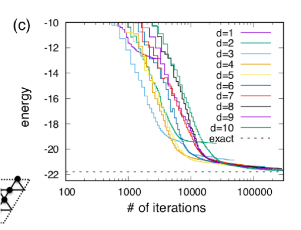
The following model is shown below.

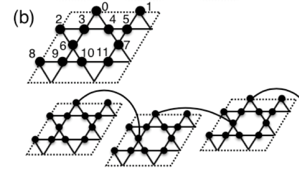
The Hamiltonian has the same shape as before, but has increased to 12 qubits, and the edges have changed as shown in the figure. The interaction is acting on the 0th and 6th qubits. The exact solution for this subsystem is $ -21.78 $, and the result calculated by Deep VQE seems to be $ -21.72 $. The energy values measured at different circuit depths are listed below.

From now on, if you connect the partial systems, it seems that $ -43.8 $ is obtained at $ N = 2 $ and $ -87.9 $ is obtained at $ N = 4 $.

Implementation

I calculated the basal energy in the case of $ N = 2 $ in model a by DeepVQE using Qulacs.

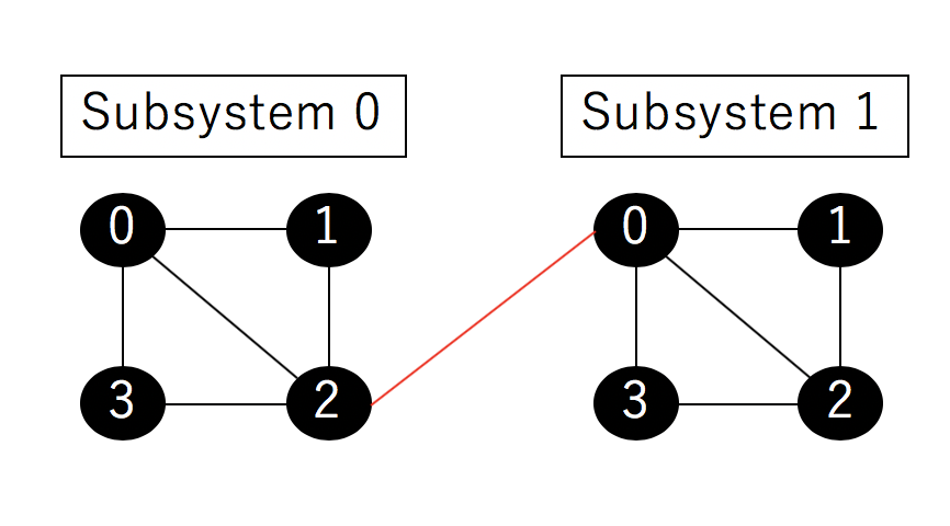
The partial Hamiltonian uses the following model as before.

\begin{align}
    \mathcal{H}_i &= \sum_{E=(\mu, \nu)}(X^{(i)}_{\mu}X^{(i)}_{\nu} + Y^{(i)}_{\mu}Y^{(i)}_{\nu} + Z^{(i)}_{\mu}Z^{(i)}_{\nu}) \\
    &= \sum_{E=(\mu, \nu)}\sum_{A=X,y,Z}A^{(i)}_{\mu} A^{(i)}_{\nu} 
\end{align}

The edges are $ E = \ {(0,1), (1,2), (2,3), (3,0), (0,2) } $ and the interaction uses:

\begin{align}
    V_{01} = \sum_{A=X,Y,Z}(A^{(i)}_{0} A^{(j)}_{2} + A^{(i)}_{2} A^{(j)}_{0})
\end{align}

Please refer to the code below when calculating the above model with Deep VQE in notebook format. The explanation is also described on the notebook.

https://github.com/Noriaki416/DeepVQE/blob/master/DeepVQE.ipynb

I'm skipping this time because I'm using BFGS to optimize the cost function and I really need to enter the gradient of the cost function. (Although it is said in the paper that you should add a gradient, I skipped it. I'm sorry.)

In addition, the results obtained using strict diagonalization are also uploaded below.

https://github.com/Noriaki416/DeepVQE/blob/master/DeepVQE_Others.ipynb

The result of the exact diagonalization is "-14.46", which matches the value in Table 1. The result of Deep VQE is also the same value, and I think that the calculation itself has been executed well.

That's it. Please point out any mistakes. If I have time, I will improve the code and try to calculate in other systems ($ N> 2 $ in model a and model b).