[PYTHON] I tried to implement multivariate statistical process management (MSPC)
- Articles sent by data scientists from the manufacturing industry
- This time, we have implemented and organized anomaly detection methods that can be used in the manufacturing industry.
Introduction
Recently, I think that the number of initiatives that utilize machine learning has begun to increase even in the manufacturing industry. This time, we have organized the multivariate statistical process management (MSPC) used in the anomaly detection project.
What is anomaly detection in the manufacturing industry?
In the manufacturing industry, there is the term preventive maintenance. Preventive maintenance refers to maintenance methods that prevent mechanical equipment failures, malfunctions, and performance degradation on the production line, and is performed for the purpose of preventing equipment from breaking and the production line from stopping. In addition, there is also operation abnormality detection to prevent the production of abnormal products from normal operation.
The anomaly detection method (MSPC) introduced this time is a method that can be used for both.
What is Multivariate Statistical Process Management (MSPC)?
When used with MSPC, the data used is only normal data for learning. Generally, when classifying by machine learning etc., it is easy to think that proper classification cannot be done unless samples of normal data and abnormal data are collected, but in the actual field, there is almost no abnormal data and it is normal. There is a lot of data only. (Actually, since it means "abnormal data = equipment failure", it is the data when the production of the factory is stopped. It is natural that there is little such data. Therefore, at the manufacturing site, we will focus on preventive maintenance. We have put it in, and we are carrying out conservation activities at a slightly excessive level.)
The basic idea of anomaly detection is to set an area where normal data exists in a multidimensional space, and when observing data that deviates from that area, it is judged as anomaly. Therefore, it is possible to build an anomaly detection model by learning only normal data.
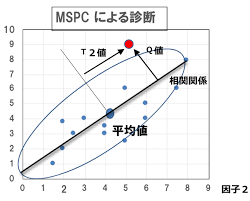
Next, we will explain how to set the management limit, which is the boundary between the normal state and the abnormal state. It's a bit amakudari, but usually there is some kind of relationship (correlation) between variables, and it is necessary to grasp the relationship between variables when properly defining the area containing normal data. In other words, you need to prepare an ellipse for two variables and a hyperelliptic for n variables. MCPC uses Principal Component Analysis (PCA) to calculate the Mahalanobis distance as a method of considering the relationships between variables. MSPC is a method of constructing a hyperelliptic curve using PCA, setting a management limit, and determining whether data deviates from it.
MSPC utilizes PCA to normalize the variance of each principal component to 1, and does not normalize all principal components to variance 1 when calculating the Mahalanobis distance. Calculate the distance from the origin by standardizing only the main principal components to variance 1. The square of this distance is called the $ Hotelling's T ^ 2 $ statistic. On the other hand, the non-major principal component is called the Q statistic (Squared Prediction Error) and is defined by the square of the distance (prediction error) from the subspace spanned by the main principal component.
Summary of MSPC
The procedure of MSPC is organized below.
- Get normal data
- Utilize PCA for normal data
- Determine the number of major principal components
- The main principal component calculates the $ T ^ 2 $ statistic, and the other principal components calculate the $ Q $ statistic.
- Set control limits for $ T ^ 2 $ statistic and $ Q $ statistic
MSPC implementation
This time, we prepared the data (sample data number: 2,756, column number: 90) for the test. We used 1000 normal data and the remaining 1,756 as evaluation data to see how much they deviated from the normal state.
The python code is below.
#Import required libraries
import pandas as pd
import numpy as np

from matplotlib import pyplot as plt
%matplotlib inline
from sklearn.preprocessing import StandardScaler
from scipy import stats
from sklearn.neighbors.kde import KernelDensity
from sklearn.decomposition import PCA

df = pd.read_csv('test_data.csv', encoding='shift_jis', header=1, index_col=0)
df.head()
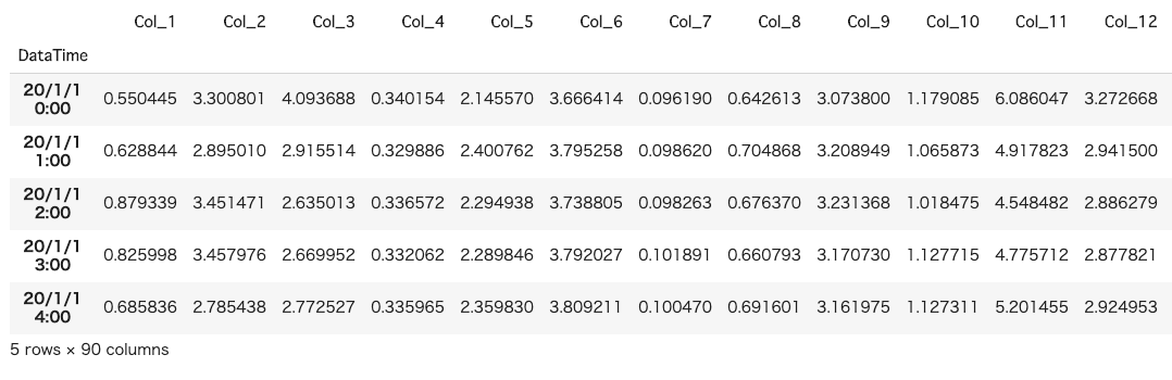
The input data looks like the above. This time, random numbers are entered in each column.
Next, we will divide the training data and evaluation data and standardize them.
#Split point
split_point = 1000
#Divided into training data (train) and evaluation data (test)
train_df = df.iloc[:(split_point-1),]
test_df = df.iloc[split_point:,]

#Standardize data
sc = StandardScaler()
sc.fit(train_df)
train_df_std = sc.transform(train_df)
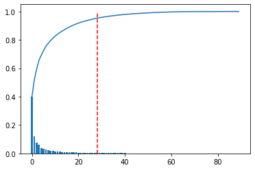
Next, perform principal component analysis to determine the main principal components. This time, the main component was the part where the cumulative contribution rate was up to 95%.
# PCA
pca = PCA()
pca.fit(train_df_std)

#Cumulative contribution graph
plt.figure()
variance = pca.explained_variance_ratio_
variance_total = np.zeros(np.shape(variance)[0])
plt.bar(range(np.shape(variance)[0]), variance)
for i in range(np.shape(variance)[0]):
    variance_total[i] = np.sum(variance[0:i+1])

plt.plot(variance_total)
NumOfScore = np.min(np.where(variance_total>0.95))
x1=[NumOfScore,NumOfScore]
y1=[0,1]
plt.plot(x1,y1,ls="--", color = "r")

pca = PCA(n_components = NumOfScore)
pca.fit(train_df_std)
Next, find the Q statistic.
#Q statistic
scores = pca.transform(train_df_std)
residuals = pca.inverse_transform(scores)-train_df_std
dist = np.sqrt(np.sum(np.power(residuals,2),axis=1))/(np.shape(train_df_std)[1])
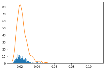
Since we have to set the control limit from normal data, we set the control limit using kernel density estimation.
#Control limit (kernel density estimation)
cr = 0.99
X = dist.reshape(np.shape(dist)[0],1)
bw= (np.max(X)-np.min(X))/100
kde = KernelDensity(kernel='gaussian', bandwidth=bw).fit(X)
X_plot = np.linspace(np.min(X), np.max(X), 1000)[:, np.newaxis]
log_dens = kde.score_samples(X_plot)
plt.figure()
plt.hist(X, bins=X_plot[:,0])
plt.plot(X_plot[:,0],np.exp(log_dens))
prob = np.exp(log_dens) / np.sum(np.exp(log_dens))
calprob = np.zeros(np.shape(prob)[0])
calprob[0] = prob[0]
for i in range(1,np.shape(prob)[0]):
    calprob[i]=calprob[i-1]+prob[i]

cl = X_plot[np.min(np.where(calprob>cr))]
Next, check when the test data does not come out of the normal data area.
#Standardize data
test_df_std = sc.transform(test_df)
# Test Data
newscores = pca.transform(test_df_std)
newresiduals = pca.inverse_transform(newscores)-test_df_std
newdist = np.sqrt(np.sum(np.power(newresiduals,2),axis=1))/(np.shape(test_df_std)[1])
Finally, set the Q statistic (including training and test data) and the control limit calculated by kernel density estimation.
#Q statistic plot
SPE = np.r_[dist,newdist]
plt.figure()
x = range(0,np.shape(df.index)[0],100)
NewTimeIndices = np.array(df.index[x])
x2 = [0, np.shape(SPE)[0]]
y2 = [cl,cl]
plt.title('SPE')
plt.plot(SPE)
plt.xticks(x,NewTimeIndices,rotation='vertical')
plt.plot(x2,y2,ls="-", color = "r")
#plt.ylim([0,1])
plt.xlabel("Time")
plt.ylabel("SPE")

# contribution plot
plt.figure()
total_residuals= np.r_[residuals,newresiduals]
CspeTimeseries = np.power(total_residuals,2)

cspe_summary=np.zeros([np.shape(CspeTimeseries)[0],10])
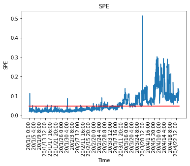
Actually, the contribution plot is calculated from here, and when the control limit is exceeded, which explanatory variable affects and becomes abnormal is calculated. You can also manage the $ T ^ 2 $ chart in the same way, and check which explanatory variables are affecting when the control limit is exceeded.
By using MSPC, it is possible to monitor sensor data with 90 variables with two control charts, and it is possible to identify which sensor is abnormal when an alarm sounds, so the monitoring load at the manufacturing site Will also go down. It is also possible to use kernel PCA instead of PCA if the relationships between variables are not linear.
finally
Thank you for reading to the end. This time, we implemented the anomaly detection method (MSPC) required at the manufacturing site. In the actual field, there are many tuning factors such as the default method of the normal state and the setting of the management limit, but I think it is better to set while operating in the field.
If you have a request for correction, we would appreciate it if you could contact us.
Recommended Posts