[PYTHON] [Français] didacticiel scikit-learn 0.18 Didacticiel d'apprentissage statistique pour le traitement des données scientifiques Mettre le tout ensemble
traduction google de http://scikit-learn.org/stable/tutorial/statistical_inference/putting_together.html Tableau du didacticiel d'apprentissage statistique pour le traitement des données scientifiques Page précédente
Mettez tout ensemble
Traitement du pipeline
Il s'avère que certains estimateurs peuvent transformer les données et certains estimateurs peuvent prédire des variables. Vous pouvez également créer des estimations combinatoires.
from sklearn import linear_model, decomposition, datasets
from sklearn.pipeline import Pipeline
from sklearn.model_selection import GridSearchCV
logistic = linear_model.LogisticRegression()
pca = decomposition.PCA()
pipe = Pipeline(steps=[('pca', pca), ('logistic', logistic)])
digits = datasets.load_digits()
X_digits = digits.data
y_digits = digits.target
###############################################################################
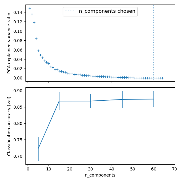
# Plot the PCA spectrum
pca.fit(X_digits)
plt.figure(1, figsize=(4, 3))
plt.clf()
plt.axes([.2, .2, .7, .7])
plt.plot(pca.explained_variance_, linewidth=2)
plt.axis('tight')
plt.xlabel('n_components')
plt.ylabel('explained_variance_')
###############################################################################
# Prediction
n_components = [20, 40, 64]
Cs = np.logspace(-4, 4, 3)
#Parameters of pipelines can be set using ‘__’ separated parameter names:
estimator = GridSearchCV(pipe,
dict(pca__n_components=n_components,
logistic__C=Cs))
estimator.fit(X_digits, y_digits)
plt.axvline(estimator.best_estimator_.named_steps['pca'].n_components,
linestyle=':', label='n_components chosen')
plt.legend(prop=dict(size=12))
Face recognition with eigenfaces
L'ensemble de données utilisé dans cet exemple est un extrait prétraité d'une «surface marquée sauvage», également appelée LFW. http://vis-www.cs.umass.edu/lfw/lfw-funneled.tgz (233MB)
"""
===================================================
Faces recognition example using eigenfaces and SVMs
===================================================
The dataset used in this example is a preprocessed excerpt of the
"Labeled Faces in the Wild", aka LFW_:
http://vis-www.cs.umass.edu/lfw/lfw-funneled.tgz (233MB)
.. _LFW: http://vis-www.cs.umass.edu/lfw/
Expected results for the top 5 most represented people in the dataset:
================== ============ ======= ========== =======
precision recall f1-score support
================== ============ ======= ========== =======
Ariel Sharon 0.67 0.92 0.77 13
Colin Powell 0.75 0.78 0.76 60
Donald Rumsfeld 0.78 0.67 0.72 27
George W Bush 0.86 0.86 0.86 146
Gerhard Schroeder 0.76 0.76 0.76 25
Hugo Chavez 0.67 0.67 0.67 15
Tony Blair 0.81 0.69 0.75 36
avg / total 0.80 0.80 0.80 322
================== ============ ======= ========== =======
"""
from __future__ import print_function
from time import time
import logging
import matplotlib.pyplot as plt
from sklearn.model_selection import train_test_split
from sklearn.model_selection import GridSearchCV
from sklearn.datasets import fetch_lfw_people
from sklearn.metrics import classification_report
from sklearn.metrics import confusion_matrix
from sklearn.decomposition import PCA
from sklearn.svm import SVC
print(__doc__)
# Display progress logs on stdout
logging.basicConfig(level=logging.INFO, format='%(asctime)s %(message)s')
###############################################################################
# Download the data, if not already on disk and load it as numpy arrays
lfw_people = fetch_lfw_people(min_faces_per_person=70, resize=0.4)
# introspect the images arrays to find the shapes (for plotting)
n_samples, h, w = lfw_people.images.shape
# for machine learning we use the 2 data directly (as relative pixel
# positions info is ignored by this model)
X = lfw_people.data
n_features = X.shape[1]
# the label to predict is the id of the person
y = lfw_people.target
target_names = lfw_people.target_names
n_classes = target_names.shape[0]
print("Total dataset size:")
print("n_samples: %d" % n_samples)
print("n_features: %d" % n_features)
print("n_classes: %d" % n_classes)
###############################################################################
# Split into a training set and a test set using a stratified k fold
# split into a training and testing set
X_train, X_test, y_train, y_test = train_test_split(
X, y, test_size=0.25, random_state=42)
###############################################################################
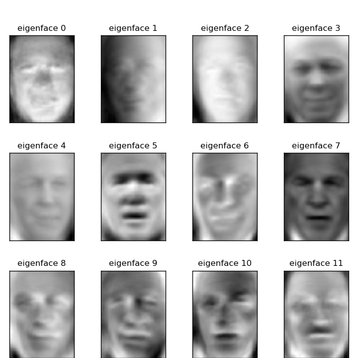
# Compute a PCA (eigenfaces) on the face dataset (treated as unlabeled
# dataset): unsupervised feature extraction / dimensionality reduction
n_components = 150
print("Extracting the top %d eigenfaces from %d faces"
% (n_components, X_train.shape[0]))
t0 = time()
pca = PCA(n_components=n_components, svd_solver='randomized',
whiten=True).fit(X_train)
print("done in %0.3fs" % (time() - t0))
eigenfaces = pca.components_.reshape((n_components, h, w))
print("Projecting the input data on the eigenfaces orthonormal basis")
t0 = time()
X_train_pca = pca.transform(X_train)
X_test_pca = pca.transform(X_test)
print("done in %0.3fs" % (time() - t0))
###############################################################################
# Train a SVM classification model
print("Fitting the classifier to the training set")
t0 = time()
param_grid = {'C': [1e3, 5e3, 1e4, 5e4, 1e5],
'gamma': [0.0001, 0.0005, 0.001, 0.005, 0.01, 0.1], }
clf = GridSearchCV(SVC(kernel='rbf', class_weight='balanced'), param_grid)
clf = clf.fit(X_train_pca, y_train)
print("done in %0.3fs" % (time() - t0))
print("Best estimator found by grid search:")
print(clf.best_estimator_)
###############################################################################
# Quantitative evaluation of the model quality on the test set
print("Predicting people's names on the test set")
t0 = time()
y_pred = clf.predict(X_test_pca)
print("done in %0.3fs" % (time() - t0))
print(classification_report(y_test, y_pred, target_names=target_names))
print(confusion_matrix(y_test, y_pred, labels=range(n_classes)))
###############################################################################
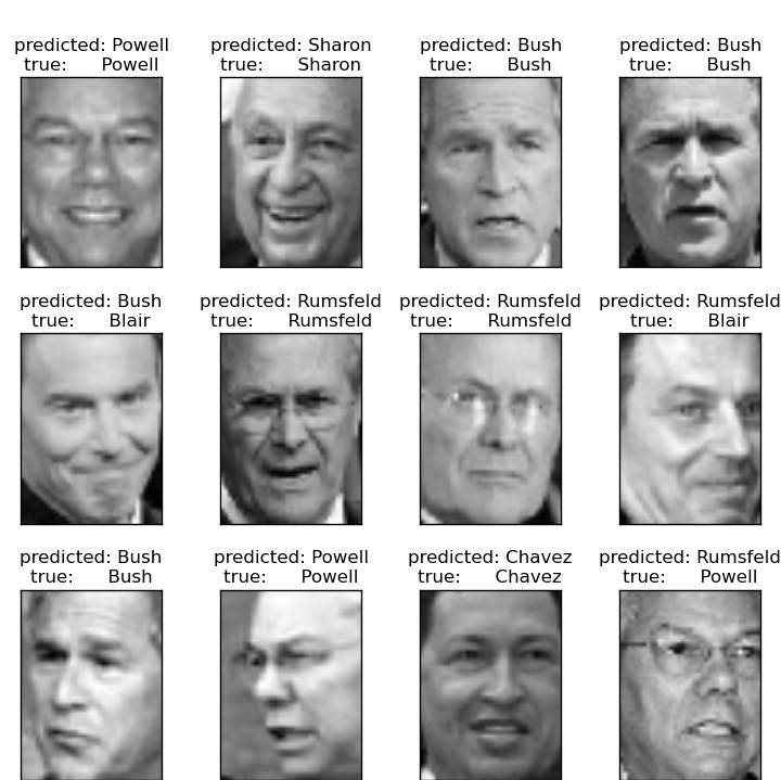
# Qualitative evaluation of the predictions using matplotlib
def plot_gallery(images, titles, h, w, n_row=3, n_col=4):
"""Helper function to plot a gallery of portraits"""
plt.figure(figsize=(1.8 * n_col, 2.4 * n_row))
plt.subplots_adjust(bottom=0, left=.01, right=.99, top=.90, hspace=.35)
for i in range(n_row * n_col):
plt.subplot(n_row, n_col, i + 1)
plt.imshow(images[i].reshape((h, w)), cmap=plt.cm.gray)
plt.title(titles[i], size=12)
plt.xticks(())
plt.yticks(())
# plot the result of the prediction on a portion of the test set
def title(y_pred, y_test, target_names, i):
pred_name = target_names[y_pred[i]].rsplit(' ', 1)[-1]
true_name = target_names[y_test[i]].rsplit(' ', 1)[-1]
return 'predicted: %s\ntrue: %s' % (pred_name, true_name)
prediction_titles = [title(y_pred, y_test, target_names, i)
for i in range(y_pred.shape[0])]
plot_gallery(X_test, prediction_titles, h, w)
# plot the gallery of the most significative eigenfaces
eigenface_titles = ["eigenface %d" % i for i in range(eigenfaces.shape[0])]
plot_gallery(eigenfaces, eigenface_titles, h, w)
plt.show()
| Prévoir | Visage unique |
|---|---|
 |
 |
Résultats attendus pour les 5 premières personnes de l'ensemble de données:
                   precision    recall  f1-score   support

Gerhard_Schroeder       0.91      0.75      0.82        28
  Donald_Rumsfeld       0.84      0.82      0.83        33
       Tony_Blair       0.65      0.82      0.73        34
     Colin_Powell       0.78      0.88      0.83        58
    George_W_Bush       0.93      0.86      0.90       129

      avg / total       0.86      0.84      0.85       282
Problème ouvert: structure de la bourse
Pouvez-vous prévoir les fluctuations du cours de l'action de Google sur une période donnée?
Structure du graphe d'apprentissage
Page suivante © 2010 --2016, développeurs scikit-learn (licence BSD).
Recommended Posts