Predict from various data in Python using Facebook Prophet, a time series prediction tool
This article is [Greg Rafferty](https://towardsdatascience.com/@raffg?source=post_page-----29810eb57e66 -------------------- ---) This is a Japanese translation of "Forecasting in Python with Facebook Prophet" published by Mr. in November 2019. .. This article is published with permission from the original author.
I'm Greg Rafferty, a data scientist in the Bay Area. You can also check the code used in this project from my github.
In this article, I'll show you how to make various predictions using the prediction library Facebook Prophet and some advanced techniques to use your expertise to handle trend inconsistencies. There are many Prophet tutorials out there on the web, but all the ways to tune Prophet's model and integrate analyst knowledge to get the model to navigate the data properly are all too detailed. not. This article will cover both.
 https://www.instagram.com/p/BaKEnIPFUq-/
A previous article on Forecasting Using Tableau (https://towardsdatascience.com/forecasting-with-python-and-tableau-dd37a218a1e5) used a modified ARIMA algorithm to passengers on commercial flights in the United States. I predicted the number. While ARIMA's approach works well for predicting stationary data and short time frames, there are some cases that ARIMA can't handle, and Facebook engineers have developed tools to use in those cases. Prophet builds its backend in STAN, a stochastic coding language. This allows Prophet to have many of the benefits of Bayesian statistics, including seasonality, inclusion of expertise, and confidence intervals that add data-driven estimates of risk.
Here, we will look at three data sources to explain how to use Prophet and its benefits. If you really want to try it at hand, install Prophet first. There is a brief description in the Facebook docs (https://facebook.github.io/prophet/docs/installation.html#python). All the code needed to build the model used to write this article can be found in this notebook. I will.
Air passenger
Let's start with the simple ones. Use the same airline passenger data used in the previous article (https://towardsdatascience.com/forecasting-with-python-and-tableau-dd37a218a1e5). Prophet requires time series data with two or more columns, the timestamp ds and the value y. After loading the data, format it as follows:
passengers = pd.read_csv('data/AirPassengers.csv')df = pd.DataFrame()
df['ds'] = pd.to_datetime(passengers['Month'])
df['y'] = passengers['#Passengers']
In just a few lines, Prophet can create a predictive model that is as sophisticated as the ARIMA model I built earlier. Here I call Prophet and make a 6-year forecast (monthly frequency, 12 months x 6 years):
prophet = Prophet()
prophet.fit(df)
future = prophet.make_future_dataframe(periods=12 * 6, freq='M')
forecast = prophet.predict(future)
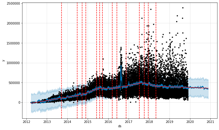
fig = prophet.plot(forecast)
a = add_changepoints_to_plot(fig.gca(), prophet, forecast)
 Number of passengers on US commercial airlines (in units of 1000)
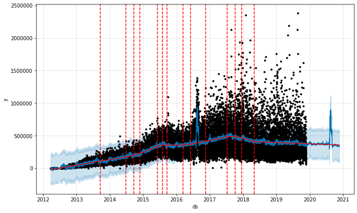
Prophet encloses the original data with black dots and displays the predictive model with a blue line. The light blue area is the confidence interval. The add_changepoints_to_plot function also adds a red line. The vertically drawn red dashed line shows where Prophet identified the trend change, and the red curve shows the trend with all seasonality removed. In this article, we will continue to use this plot format.
That's it for the simple case, and now let's look at some more complex data.
Divvy Bike Share
Divvy is a bicycle sharing service in Chicago. I have previously worked on a project that analyzed Divvy data and associated it with weather information gathered from Weather Underground. I knew this data showed strong seasonality, so I chose it because I thought it would be a great example of demonstrating Prophet's capabilities.
Divvy data is sorted by ride. To format the data for Prophet, first sum up to the daily level and then the daily "events" column mode (for example, as an example of weather conditions: "unclear" "rain or snow" "sunny" "sunny" Create a column consisting of "cloudy", "storm", "unknown", etc.), number of uses (rides), and average temperature.
Once you've formatted your data, let's take a look at how many times it's used per day:

From this we can see that the data has a clear seasonality and the trend is increasing over time. We will use this dataset to describe how to add additional regressors, in this case weather and temperature. Let's see the temperature:

It is very similar to the previous graph, but there is no upward trend. This similarity makes sense because more people ride their bikes on sunny and warm days, and both plots move up and down in tandem.
When you add another external explanatory variable to create a forecast, the external variable you add requires forecast period data. For this reason, I've shortened Divvy's data by a year so that I can predict that year along with the weather information. You can also see that Prophet has added the default US holidays.
prophet = Prophet()
prophet.add_country_holidays(country_name='US')
prophet.fit(df[d['date'] < pd.to_datetime('2017-01-01')])
future = prophet.make_future_dataframe(periods=365, freq='d')
forecast = prophet.predict(future)
fig = prophet.plot(forecast)
a = add_changepoints_to_plot(fig.gca(), prophet, forecast)
plt.show()
fig2 = prophet.plot_components(forecast)
plt.show()
The code block above creates the trend plot described in the Air Passenger section.
 Divvy trend plot
And here is the component plot:
 Divvy component plot
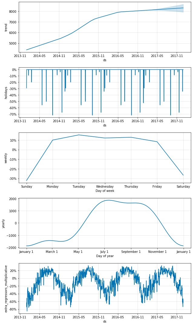
The component plot consists of three sections: Trends, Holidays, and Seasonality. The sum of these three components actually makes up the entire model. Trends are the data after subtracting all other components. The holiday plot shows the impact of all the holidays in the model. The holidays implemented in Prophet can be seen as an unnatural event, where the trend deviates from the baseline but returns after the event ends. External explanatory variables (more on this later) are similar to holidays in that they can cause the trend to deviate from the baseline, but the trend remains unchanged after the event. In this case, all holidays have led to a decrease in passenger numbers, which also makes sense given that many of our users are commuters. Looking at the weekly seasonal component, we can see that the number of users is fairly constant throughout the week, but declines sharply on weekends. This provides further evidence to support the speculation that most passengers are commuters. Last but not least, the graph of seasonal variation over the year is quite wavy. These plots are made up of Fourier transforms, essentially stack sine waves. Obviously, the default value in this case is too flexible. To smooth the curve, we now create a Prophet model to turn off the seasonality of the year and add external variables to accommodate it, but with less freedom. The model also adds these weather variables.
prophet = Prophet(growth='linear',
                  yearly_seasonality=False,
                  weekly_seasonality=True,
                  daily_seasonality=False,
                  holidays=None,
                  seasonality_mode='multiplicative',
                  seasonality_prior_scale=10,
                  holidays_prior_scale=10,
                  changepoint_prior_scale=.05,
                  mcmc_samples=0
                 ).add_seasonality(name='yearly',
                                    period=365.25,
                                    fourier_order=3,
                                    prior_scale=10,
                                    mode='additive')prophet.add_country_holidays(country_name='US')
prophet.add_regressor('temp')
prophet.add_regressor('cloudy')
prophet.add_regressor('not clear')
prophet.add_regressor('rain or snow')
prophet.fit(df[df['ds'] < pd.to_datetime('2017')])
future = prophet.make_future_dataframe(periods=365, freq='D')
future['temp'] = df['temp']
future['cloudy'] = df['cloudy']
future['not clear'] = df['not clear']
future['rain or snow'] = df['rain or snow']
forecast = prophet.predict(future)
fig = prophet.plot(forecast)
a = add_changepoints_to_plot(fig.gca(), prophet, forecast)
plt.show()
fig2 = prophet.plot_components(forecast)
plt.show()
The trend plots were pretty much the same, so I'll just show you the component plots:
 Divvy component plot with smoothed curves and added external variables for annual seasonality and weather
In this plot, the last year of the trend is up, not down like the first plot! This can be explained by the fact that the average temperature in the data last year was low and the number of users decreased more than expected. Also, the annual curve has been smoothed and an extra_regressors_multiplicative plot has been added. This shows the effect of the weather. The increase / decrease in the number of users is also as expected. The number of users increases in the summer and decreases in the winter, many of which can be explained by the weather. There is one more thing I would like to confirm for the demonstration. Run the above model again, this time adding only the rain and snow external variables. The component plot looks like this:
 Divvy component plot showing only the effects of rain and snow
This shows that on rainy or snowy days, the number of daily usages is about 1400 less than on non-rainy days. It ’s pretty interesting, is n’t it?
Finally, we aggregate this dataset by the hour to create another component plot, the daily seasonality. The plot looks like this:
 Divvy component plot showing daily seasonality
As Rivers says, 4am is the worst time to get up in the morning. Apparently Chicago cyclists agree. After 8 am, the morning commuter peaks. And around 6 pm, the whole peak will come by the returnees in the evening. You can also see that there is a small peak after midnight. Probably due to those returning home from the bar. That's the Divvy data! Next, let's move on to Instagram.
Prophet was originally designed by Facebook to analyze its data. Then this dataset is a great place to try Prophet. I searched Instagram for accounts with some interesting trends and found three accounts: @natgeo, @kosh_dp //www.instagram.com/kosh_dp/), @ jamesrodriguez10
National Geographic
 https://www.instagram.com/p/B5G_U_IgVKv/
In 2017, when I was working on a project, I was working on a National Geographic [Instagram account](https: // I noticed that there is an anomaly at www.instagram.com/natgeo/). In August 2016, there was an incident where the number of likes per photo mysteriously suddenly increased dramatically and returned to baseline as soon as August ended. I wanted to model this surge as a result of a month-long marketing campaign to increase the number of likes and see if I could predict the effectiveness of future marketing campaigns.
Here are the number of likes for National Geographic: Trends are clearly increasing and variability is increasing over time. There are many exceptions to the dramatic number of likes, but in the August 2016 Spike, all photos posted that month were overwhelmingly more likes than those posted in the months before and after. I have won the number.

I don't want to guess why this is, but let's assume that for this model we've created, for example, National Geographic's marketing department has run a one-month campaign specifically aimed at increasing likes. Let's look. First, build a model that ignores this fact and create a baseline for comparison.
 Number of likes per photo of National Geographic
Prophet seems to be confused by this spike. You can see that we are trying to add this spike to the seasonal component of each year, as shown by the blue line for the August surge each year. Prophet wants to call this a recurring event. Let's make a holiday this month to tell Prophet that something special happened in 2016 that wasn't repeated in other years:
promo = pd.DataFrame({'holiday': "Promo event",
                      'ds' : pd.to_datetime(['2016-08-01']),
                      'lower_window': 0,
                      'upper_window': 31})
future_promo = pd.DataFrame({'holiday': "Promo event",
                      'ds' : pd.to_datetime(['2020-08-01']),
                      'lower_window': 0,
                      'upper_window': 31})promos_hypothetical = pd.concat([promo, future_promo])
The promo data frame contains only the August 2016 event, and the promos_hypothetical data frame contains additional promotions that National Geographic assumes to be implemented in August 2020. When adding holidays, Prophet allows you to include more or less days in basic holiday events, such as whether Black Friday is included in Thanksgiving or Christmas Eve is included in Christmas. can also do. This time I added 31 days after "holiday" to include the entire month in the event. Below is the code and the new trend plot. Note that we specified holidays = promo when calling the Prophet object.
prophet = Prophet(holidays=promo)
prophet.add_country_holidays(country_name='US')
prophet.fit(df)
future = prophet.make_future_dataframe(periods=365, freq='D')
forecast = prophet.predict(future)
fig = prophet.plot(forecast)
a = add_changepoints_to_plot(fig.gca(), prophet, forecast)
plt.show()
fig2 = prophet.plot_components(forecast)
plt.show()
 Number of likes per photo of National Geographic, including the August 2016 marketing campaign
It is wonderful! Here Prophet shows that this ridiculous surge in likes has certainly surged only in 2016, not in August each year. So let's take this model again and use the promos_hypothetical data frame to predict what would happen if National Geographic launched the same campaign in 2020.
 Number of likes per photo of National Geographic assuming a marketing campaign in 2020
You can use this method to predict what happens when you add an unnatural event. For example, this year's product sales plan may be a model. Now let's move on to the next account.
Anastasia Kosh
 https://www.instagram.com/p/BfZG2QCgL37/
Anastasia Kosh is a Russian photographer who posts wacky self-portraits on her Instagram and music videos on YouTube. When I lived in Moscow a few years ago, we lived on the same street and were neighbors. At the time, her Instagram had about 10,000 followers, but in 2017 YouTube accounts spread rapidly in Russia, making her a little celebrity, especially among teens in Moscow. Her Instagram account has grown exponentially and her followers are rapidly approaching one million, and I thought this exponential growth would be a perfect challenge for Prophet.
The data to model is:
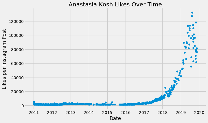
This is a typical hockey stick and shows optimistic growth, but only in this case would it really be! As with any other data we've seen so far, modeling with linear growth gives unrealistic predictions.
 Linear growing Anastasia Kosh likes per photo
This curve continues infinitely. But, of course, there is a limit to the number of Instagram likes. Theoretically, this limit is equal to the total number of registered accounts on the service. But the reality is that not all accounts see photos, and they don't like them. This is where a little expertise as an analyst comes in handy. This time I decided to model this with logistic growth. To do this, you need to tell Prophet the upper limit ceiling (Prophet calls it cap) and the lower limit floor.
cap = 200000
floor = 0
df['cap'] = cap
df['floor'] = floor
After my knowledge of Instagram and a little trial and error, I decided to limit the number of likes to 200,000 and the lower limit to 0. In Prophet, these values can be defined as a function of time and do not have to be constants. In this case, you really need a constant value:
prophet = Prophet(growth='logistic',
                  changepoint_range=0.95,
                  yearly_seasonality=False,
                  weekly_seasonality=False,
                  daily_seasonality=False,
                  seasonality_prior_scale=10,
                  changepoint_prior_scale=.01)
prophet.add_country_holidays(country_name='RU')
prophet.fit(df)
future = prophet.make_future_dataframe(periods=1460, freq='D')
future['cap'] = cap
future['floor'] = floor
forecast = prophet.predict(future)
fig = prophet.plot(forecast)
a = add_changepoints_to_plot(fig.gca(), prophet, forecast)
plt.show()
fig2 = prophet.plot_components(forecast)
plt.show()
I have now defined this growth as logistical growth, turning off all seasonality (it doesn't seem to be that much in this plot) and adjusting some more parameters. Since most of Anastasia's followers are in Russia, I also added Russia's default holidays. When you call the .fit method with df, Prophet looks at the cap and floor columns of df and recognizes that they should be included in the model. At this time, let's add these columns to the data frame when creating the prediction data frame (future data frame of the above code block). This will be explained again in the next section. But for now, the trend plot is much more realistic!
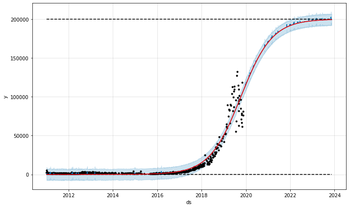 Logistic Growth Anastasia Kosh Likes Per Photo
Let's look at the last example.
James Rodríguez
 https://www.instagram.com/p/BySl8I7HOWa/
James Rodríguez is a Colombian footballer who played great in both the 2014 and 2018 World Cups. His Instagram account has grown steadily since its opening. However, while working on Previous Analysis, during the last two World Cups, his I noticed a rapid and sustained increase in followers on my account. In contrast to National Geographic's account surge, which can be modeled as a holiday season, Rodríguez's growth hasn't returned to baseline after two tournaments and is redefining a new baseline. This is a radically different move, and capturing this move requires a different modeling approach.
Below are the number of likes per photo since the James Rodríguez account was opened:

It's difficult to model this neatly with the techniques we've used so far in this tutorial. The trend baseline increased at the first World Cup in the summer of 2014, spikes occurred at the second World Cup in the summer of 2018, and the baseline may have changed. Attempting to model this behavior with the default model does not work.
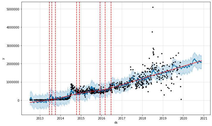 Number of likes per photo of James Rodríguez
That said, it's not a terrible model. It's just that the behavior in these two World Cups isn't well modeled. If you model these tournaments as holidays, as in the Anastasia Kosh data above, you'll see improvements in the model.
wc_2014 = pd.DataFrame({'holiday': "World Cup 2014",
                      'ds' : pd.to_datetime(['2014-06-12']),
                      'lower_window': 0,
                      'upper_window': 40})
wc_2018 = pd.DataFrame({'holiday': "World Cup 2018",
                      'ds' : pd.to_datetime(['2018-06-14']),
                      'lower_window': 0,
                      'upper_window': 40})world_cup = pd.concat([wc_2014, wc_2018])prophet = Prophet(yearly_seasonality=False,
                  weekly_seasonality=False,
                  daily_seasonality=False,
                  holidays=world_cup,
                  changepoint_prior_scale=.1)
prophet.fit(df)
future = prophet.make_future_dataframe(periods=365, freq='D')
forecast = prophet.predict(future)
fig = prophet.plot(forecast)
a = add_changepoints_to_plot(fig.gca(), prophet, forecast)
plt.show()
fig2 = prophet.plot_components(forecast)
plt.show()
 Number of likes per photo of James Rodríguez when adding holidays during the World Cup
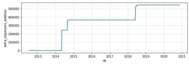
It's too late for the model to respond to the changing trend lines, especially in the 2014 World Cup, and I personally don't like it yet. The trend line transition is too smooth. In such cases, you can make Prophet consider sudden changes by adding an external explanatory variable.
In this example, each tournament defines two periods, pre-tournament and post-convention. By modeling this way, we assume that there is a specific trend line in front of the tournament, that trend line will undergo a linear change during the tournament, followed by a different trend line after the tournament. .. I define these periods as 0 or 1, on or off and let Prophet train the data to learn its magnitude.
df['during_world_cup_2014'] = 0
df.loc[(df['ds'] >= pd.to_datetime('2014-05-02')) & (df['ds'] <= pd.to_datetime('2014-08-25')), 'during_world_cup_2014'] = 1
df['after_world_cup_2014'] = 0
df.loc[(df['ds'] >= pd.to_datetime('2014-08-25')), 'after_world_cup_2014'] = 1df['during_world_cup_2018'] = 0
df.loc[(df['ds'] >= pd.to_datetime('2018-06-04')) & (df['ds'] <= pd.to_datetime('2018-07-03')), 'during_world_cup_2018'] = 1
df['after_world_cup_2018'] = 0
df.loc[(df['ds'] >= pd.to_datetime('2018-07-03')), 'after_world_cup_2018'] = 1
Update future dataframes to include "holiday" events as follows:
prophet = Prophet(yearly_seasonality=False,
                  weekly_seasonality=False,
                  daily_seasonality=False,
                  holidays=world_cup,
                  changepoint_prior_scale=.1)prophet.add_regressor('during_world_cup_2014', mode='additive')
prophet.add_regressor('after_world_cup_2014', mode='additive')
prophet.add_regressor('during_world_cup_2018', mode='additive')
prophet.add_regressor('after_world_cup_2018', mode='additive')prophet.fit(df)
future = prophet.make_future_dataframe(periods=365)future['during_world_cup_2014'] = 0
future.loc[(future['ds'] >= pd.to_datetime('2014-05-02')) & (future['ds'] <= pd.to_datetime('2014-08-25')), 'during_world_cup_2014'] = 1
future['after_world_cup_2014'] = 0
future.loc[(future['ds'] >= pd.to_datetime('2014-08-25')), 'after_world_cup_2014'] = 1future['during_world_cup_2018'] = 0
future.loc[(future['ds'] >= pd.to_datetime('2018-06-04')) & (future['ds'] <= pd.to_datetime('2018-07-03')), 'during_world_cup_2018'] = 1
future['after_world_cup_2018'] = 0
future.loc[(future['ds'] >= pd.to_datetime('2018-07-03')), 'after_world_cup_2018'] = 1forecast = prophet.predict(future)
fig = prophet.plot(forecast)
a = add_changepoints_to_plot(fig.gca(), prophet, forecast)
plt.show()
fig2 = prophet.plot_components(forecast)
plt.show()
 Number of likes per photo of James Rodríguez with external explanatory variables added
Look at this blue line. The red line shows trends only and is excluded from the effects of additional external variables and holidays. See how the blue trendline soars during the World Cup. This is exactly what our expertise teaches! When Rodríguez scored his first goal at the World Cup, suddenly thousands of followers gathered on his account. You can see the concrete effect of these external explanatory variables by looking at the component plot.
 Component plot of James Rodríguez World Cup external explanatory variables
This shows that the World Cup had no effect on the number of likes of Rodríguez's photos in 2013 or early 2014. During the 2014 World Cup, his average rose dramatically as shown in the image, which continued after the tournament (which he got so many active followers during this event). I can explain from that). There was a similar increase at the 2018 World Cup, but not so dramatically. It can be inferred that this is probably because there weren't many football fans left at that time who didn't know him.
Thank you for following this article to the end! You should now understand how to use holidays in Prophet, linear and logistic growth, and how to use external explanatory variables to significantly improve Prophet's predictions. Facebook has created an incredibly useful tool called Prophet, turning the once very difficult task of stochastic prediction into a simple set of parameters that can be broadly tuned. May your predictions be great!
Translation cooperation
Original Author: Greg Rafferty Thank you for letting us share your knowledge!
This article was published with the cooperation of the following people. Thank you again. Selector: yumika tomita Translator: siho1 Auditor: takujio Publisher: siho1
Would you like to write an article with us?
We translate high-quality articles from overseas into Japanese with the cooperation of several excellent engineers and publish the articles. Please contact us if you can sympathize with the activity or if you are interested in spreading good articles to many people. Please send a message with the title "I want to participate" in [Mail](mailto: [email protected]), or send a message in Twitter. For example, we can introduce the parts that can help you after the selection.
- We will always reply to your message.
We look forward to your opinions and impressions.
How was this article? ・ I wish I had done this, I want you to do more, I think it would be better ・ This kind of place was good We are looking for frank opinions such as. Please feel free to post in the comments section as we will use your feedback to improve the quality of future articles. We also welcome your comments on Twitter. We look forward to your message.
Recommended Posts