[PYTHON] Inverted pendulum with model predictive control

I tried model prediction control using cvxpy, which is one of the optimization modules of Python. As a subject, I chose an inverted pendulum, which is not an exaggeration to say that the control system is Hello, World !.

Model predictive control and inverted pendulum

Basically, the sample code on the following site is the main.

Model Predictive Control and Sample Code

By the way, the inverted pendulum handled this time is [Inverted pendulum] of Wikipedia (https://ja.wikipedia.org/wiki/%E5%80%92%E7%AB%8B%E6%8C%AF%E5%AD%90 ) Is assumed to be a dolly-driven inverted pendulum. The equation of motion is as follows. Each variable is basically unified with the Wikipedia article, but only F and u are different.

(M + m)\ddot{x} - ml\ddot{\theta}cos\theta + ml\dot{\theta}^2sin\theta = u \\
l\ddot{\theta} - gsin\theta = \ddot{x}cos\theta

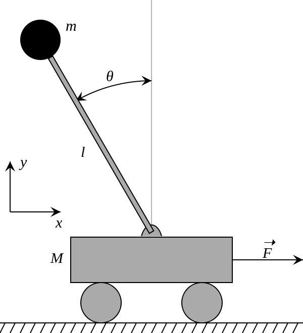
Approximation is made based on the assumption that θ is close to 0, and the model is represented by a linear equation.

\frac{d}{dt}
\begin{pmatrix}
x \\
\dot{x} \\
\theta \\
\dot{\theta}
\end{pmatrix}
=
\begin{pmatrix}
0 & 1 & 0 & 0 \\
0 & 0 & \frac{mg}{M} & 0 \\
0 & 0 & 0 & 1 \\
0 & 0 & \frac{(M + m)g}{lM} & 0
\end{pmatrix}
\begin{pmatrix}
x \\
\dot{x} \\
\theta \\
\dot{\theta}
\end{pmatrix}
+
\begin{pmatrix}
0 \\
\frac{1}{M} \\
0 \\
\frac{1}{lM}
\end{pmatrix}
u

A = 
\begin{pmatrix}
0 & 1 & 0 & 0 \\
0 & 0 & \frac{mg}{M} & 0 \\
0 & 0 & 0 & 1 \\
0 & 0 & \frac{(M + m)g}{lM} & 0
\end{pmatrix}
Δt
+
\begin{pmatrix}
1 & 0 & 0 & 0 \\
0 & 1 & 0 & 0 \\
0 & 0 & 1 & 0 \\
0 & 0 & 0 & 1
\end{pmatrix} \\
B =
\begin{pmatrix}
0 \\
\frac{1}{M} \\
0 \\
\frac{1}{lM}
\end{pmatrix}
Δt

{\bf x}_{t+1} = A{\bf x}_{t} + Bu

Δt is the control cycle. If Δt is 0.1 [s], the control input will be changed every 0.1 seconds based on the current state.

code

Define the linear equations as follows:

mpc.py

import time
from cvxpy import *
import numpy as np
import matplotlib.pyplot as plt

n_state = 4   #Number of states
m_state = 1   #Number of control inputs
T = 100  #Decide how many steps to predict

#simulation parameter
delta_t = 0.01

M = 1.0  # [kg]
m = 0.3  # [kg]
g = 9.8  # [m/s^2]
l = 0.6  # [m]

# Model Parameter
A = np.array([
	[0.0, 1.0, 0.0, 0.0],
	[0.0, 0.0, m * g / M, 0.0],
	[0.0, 0.0, 0.0, 1.0],
	[0.0, 0.0, g * (M + m) / (l * M), 0.0]
	])
A = np.eye(n_state) + delta_t * A

B = np.array([
	[0.0],
	[1.0 / M],
	[0.0],
	[1.0 / (l * M)]
	])
B = delta_t * B

#Initial state of inverted pendulum
#This time we aim for everything to converge to 0
x_0 = np.array([
	[-0.02],
	[0.0],
	[0.02],
	[0.0]
	])

x = Variable(n_state, T+1)
u = Variable(m_state, T)

The code below actually defines the cost function and optimizes it. Use cost_arr to adjust the weight for each state. The code around here is almost just copied from Model Predictive Control and Sample Code.

mpc.py

cost_arr = np.array([
	[1.0, 0.0, 0.0, 0.0],
	[0.0, 1.0, 0.0, 0.0],
	[0.0, 0.0, 0.1, 0.0],
	[0.0, 0.0, 0.0, 0.1]
	])

states = []
for t in range(T):
    #Find an array u that reduces the value of the cost function
    cost = sum_squares(cost_arr*x[:,t+1]) + sum_squares(0.1*u[:,t])
    #Give constraint equations (linear equations and control input limits)
    constr = [x[:,t+1] == A*x[:,t] + B*u[:,t],
    			norm(u[:,t], 'inf') <= 20.0]
    states.append( Problem(Minimize(cost), constr) )
# sums problem objectives and concatenates constraints.
prob = sum(states)
#Add two more constraints
#Last state(State after T step)Is all 0, that is, the ideal state
#And since the current state x0 is a fact, it becomes a constraint.
prob.constraints += [x[:,T] == 0, x[:,0] == x_0]

start = time.time()
result=prob.solve(verbose=True)
elapsed_time = time.time() - start
print("calc time:{0} [sec]".format(elapsed_time))

#If it diverges, it ends as out of control
if result == float("inf"):
    print("Cannot optimize")
    import sys
    sys.exit()

By the way, the above code is equivalent to one control. Since control is always performed, the inverted pendulum can be kept standing without falling by repeating the above process.

The code for iterative model predictive control is as follows.

mpc.py

cnt = 0
#Control 1000 times
while cnt < 1000:
    states = []
    for t in range(T):
        cost = sum_squares(cost_arr*x[:,t+1]) + sum_squares(0.1*u[:,t])
        constr = [x[:,t+1] == A*x[:,t] + B*u[:,t],
                    norm(u[:,t], 'inf') <= 20.0]
        states.append( Problem(Minimize(cost), constr) )
    # sums problem objectives and concatenates constraints.
    prob = sum(states)
    prob.constraints += [x[:,T] == 0, x[:,0] == x_0]

    start = time.time()
    result=prob.solve(verbose=False)
    elapsed_time = time.time() - start

    if result == float("inf"):
        print("Cannot optimize")
        import sys
        sys.exit()

    #Get an array of optimal control inputs
    good_u_arr = np.array(u[0,:].value[0,:])[0]
    
    #Enter the control input and get the next state
    #I don't think about noise this time
    x_next = np.dot(A, x_0) + B * good_u_arr[0]
    x_0 = x_next

    cnt += 1

    #From left to right x(Position of the dolly), \dot{x}(Bogie speed), rad(Pendulum angle), \dot{rad}(Angular velocity of the pendulum)
    print(x_next.reshape(-1))

It often goes out of control depending on the initial state of the inverted pendulum.

While model predictive control has high control performance, it seems to have the problem of a large amount of calculation. My PC has also warmed up considerably.