Explain what is stochastic gradient descent by running it in Python

What is the gradient descent method used for?

Gradient descent is often used in statistics and machine learning. In particular, machine learning often results in numerically solving a problem that basically minimizes (maximizes) some function. (E.g. Least squares method → Minimize the sum of squares of error (Reference), Neural network parameter determination etc ...)

So, basically, it's a problem to find a place where it is differentiated and becomes 0, differentiated to 0. So, this gradient descent method is important when solving the programmatically what is the value that is differentiated to 0. There are several types of gradient descent, but here we will deal with the steepest descent method and the stochastic gradient descent method. First of all, I would like to check with a one-dimensional graph to get an image.

For one dimension

In the one-dimensional case, there is no concept of stochastic, it is just a gradient descent method. (What do you mean later) For the one-dimensional example, let's use the one with the normal distribution minus. The graphs of $ x_ {init} = 0 $ and $ x_ {init} = 6 $ are used as examples. The target graph is the one in which the density function of the normal distribution is subtracted and turned downward.

** Graph with initial value = 0 ** You can see that it starts from the end of the graph and converges at the minimum value at the smallest point. The blue line graph is the minus version of the normal distribution, and the green line graph is the differential value graph.

** Graph with initial value = 6 **

Determine the next $ x $ value based on the slope at each point, check the slope at that position, and then descend, and so on to reach the minimum value (actually the minimum value). In the above example, as the value approaches the minimum value, the slope becomes gentle, so the amount of progress in one step gradually decreases, and when it becomes smaller than a certain standard, it stops. I will.

The code that wrote these two graphs is here.

2D (quadratic function)

In the case of multidimensional, it will descend considering the direction to proceed to the next step. The characteristics of the movement change depending on the target function, but first I drew a graph using the quadratic function $ Z = -3x ^ 2-5y ^ 2 + 6xy $ as an example. You can see it moving toward the top while moving in a zigzag manner.

The code is here

For 2D

In the case of 2D (2D normal distribution)

It was found that when the steepest descent method is applied to a two-dimensional normal distribution (minus), it does not move in a zigzag manner and descends to the minimum value neatly. I would like to investigate the difference in the state of convergence depending on the target function.

The code is here

How the steepest descent method works

The mechanism of the steepest descent method is to select the starting point first, and then the vector with the largest descent slope at that point, that is,

\nabla f = \frac{d f({\bf x})}{d {\bf x}} = \left[ \begin{array}{r} \frac{\partial f}{\partial x_1} \\ ... \\ \frac{\partial f}{\partial x_2} \end{array} \right]

Is the way to go to the next step using. In the graph above, this gradient vector multiplied by the learning rate $ \ eta $ is represented by a straight line. So

x_{i+1} = x_i - \eta \nabla f

The process of repeating this step until it converges is performed.

What is stochastic gradient descent?

Now, let's move on to stochastic gradient descent. First of all, I would like to explain the target function using the error function of the regression line that was used in Explanation of regression analysis. There is a part that changes the interpretation a little (using the maximum likelihood method), so [end of sentence](http://qiita.com/kenmatsu4/items/d282054ddedbd68fecb0#http://qiita.com/kenmatsu4/items/d282054ddedbd68fecb0# Supplement The parameters of the regression line are calculated by the maximum likelihood method) as a supplement.

Data is,

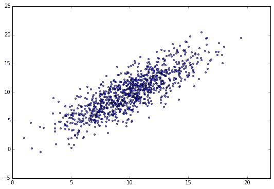
y_n = \alpha x_n + \beta + \epsilon_n　　　(\alpha=1, \beta=0)\\
\epsilon_n ∼ N(0, 2)　　　　　　　　　　　　　　　　

Let's use the example of preparing N = 1000 data sets and finding the regression line. The scatter plot is as follows.

Error function,

E({\bf w})=\sum_{n=1}^{N} E_n({\bf w}) = \sum_{n=1}^{N} (y_n -\alpha x_n - \beta)^2 \\
{\bf w} = (\alpha, \beta)^{\rm T}　　　　　　　　　　　　　　　　　　　　　　　

We will find the minimum value of, but first, in order to calculate the gradient, we derive the gradient vector partially differentiated by $ \ alpha and \ beta $, respectively.

\frac{\partial E({\bf w})}{\partial \alpha} = \sum_{n=1}^{N} \frac{\partial E_n({\bf w})}{\partial \alpha} = 
\sum_{n=1}^N (2 x_n^2  \alpha +  2 x_n \beta - 2 x_n y_n )\\

\frac{\partial E({\bf w})}{\partial \beta} = \sum_{n=1}^{N}\frac{\partial E_n({\bf w})}{\partial \alpha} =
\sum_{n=1}^N (2\beta + 2  x_n \alpha - 2y_n)　　　

So the gradient vector is

\nabla E({\bf w}) = \frac{d E({\bf w}) }{d {\bf w}} = \left[ \begin{array}{r} \frac{\partial E({\bf w})}{\partial \alpha} \\ \frac{\partial E({\bf w})}{\partial \beta} \end{array} \right] = \sum_{n=1}^{N}
\nabla E_n({\bf w}) = \sum_{n=1}^{N} \left[ \begin{array}{r} \frac{\partial E_n({\bf w})}{\partial \alpha} \\ \frac{\partial E_n({\bf w})}{\partial \beta} \end{array} \right]=
\left[ \begin{array}{r} 
2 x_n^2  \alpha +  2 x_n \beta - 2 x_n y_n \\ 
2\beta + 2  x_n \alpha - 2y_n 　
\end{array} \right]

It will be.

Since it is a problem to find a simple regression line, it may be solved as an equation, but we will solve this using the stochastic gradient descent method. Instead of using all N = 1000 data here, the key to this method is to calculate the gradient for the data randomly sampled from here and determine the next step.

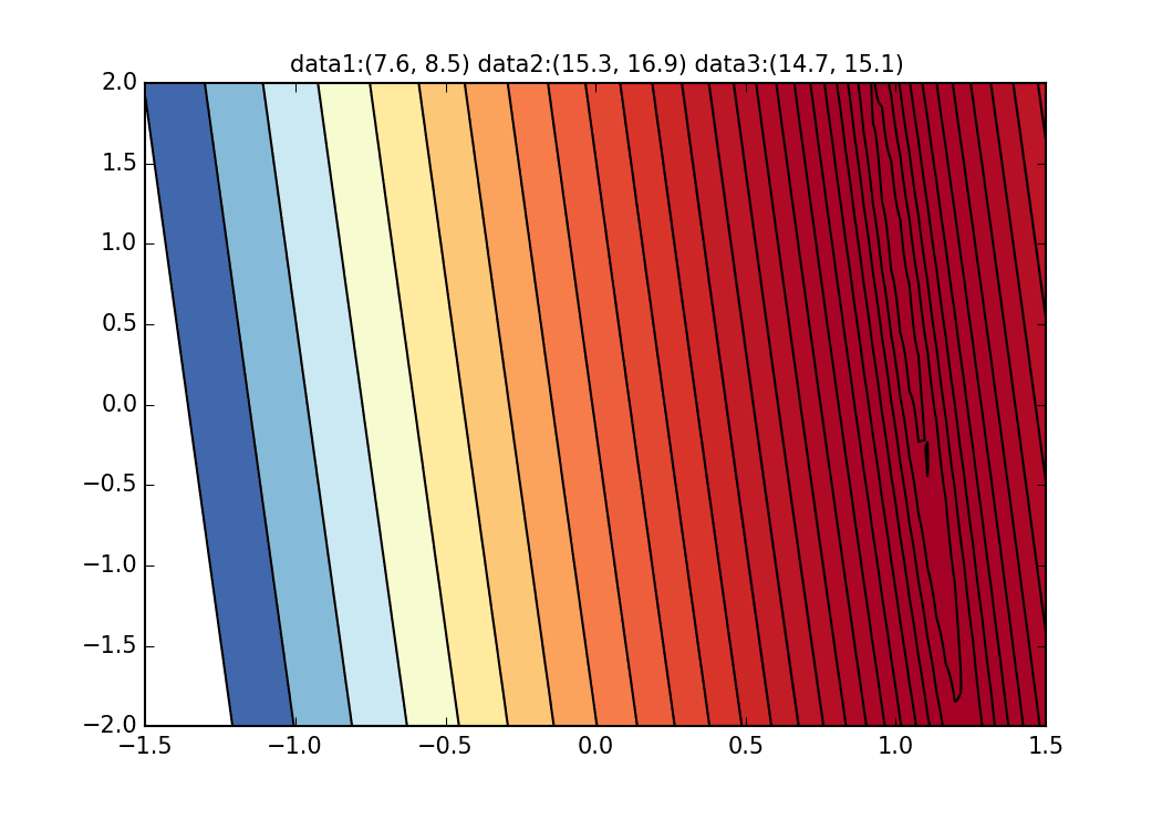
First, let's randomly extract 20 pieces from this data set and make a graph. The horizontal axis is $ \ alpha $, the vertical axis is $ \ beta $, and the Z axis is the error $ E (\ alpha, \ beta) $.

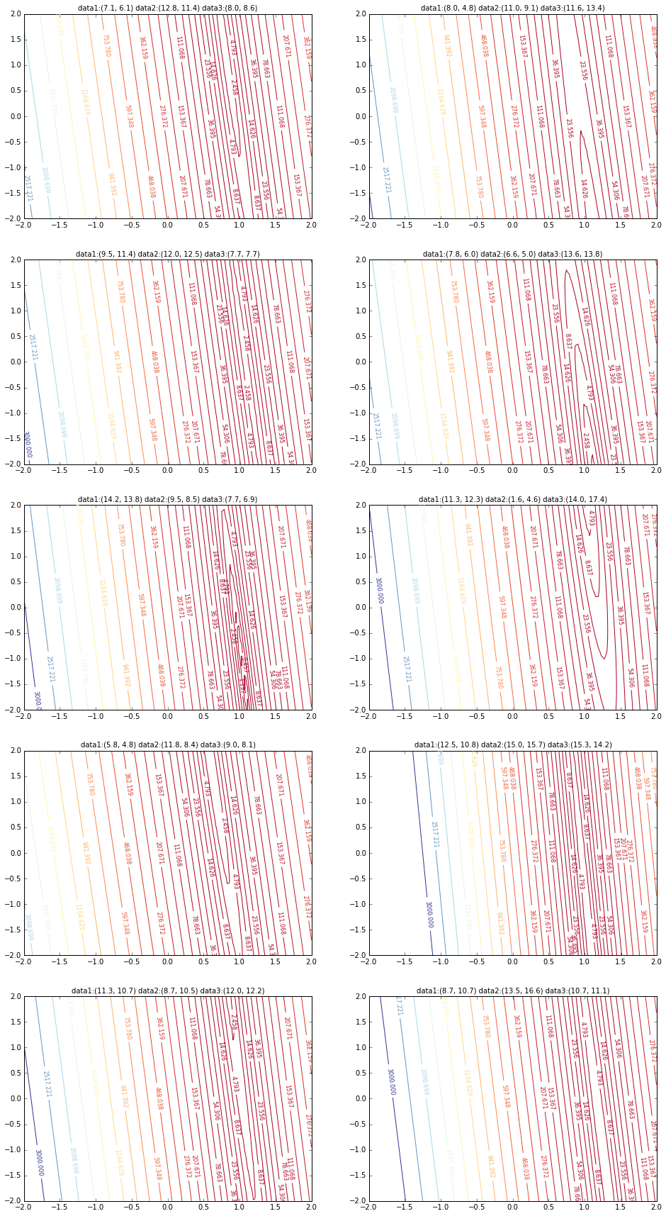
I think that the minimum values of the graph are scattered around $ \ alpha = 1, \ beta = 0 $. This time, I randomly picked up 3 data from 1000 data and wrote this graph based on it. The initial value is $ \ alpha = -1.5, \ beta = -1.5 $, the learning rate is proportional to the reciprocal of the number of iterations $ t $, and the reciprocal of $ E (\ alpha, \ beta) $ at that point is also multiplied. I tried using the one. It seems that there is no choice but to make trial and error about how to determine this learning rate and initial value, but if anyone knows a good way to look for it, I would be grateful if you could tell me. If you make a mistake a little, the dots will fly out of the frame and will not come back (laughs).

Since the error function that determines the gradient depends on the random number, it can be seen that it changes every time. The regression line is also quite violent at first, but you can see that it gradually becomes quieter and converges.

The code is here.

To be honest, the above animation example is for the one with better convergence, and the graph below shows the convergence of $ \ alpha $ and $ \ beta $ when repeated 10000 times, but $ \ alpha $ is approaching the true value of 1, but $ \ beta $ converges around 0.5 and is unlikely to approach the true value of 0 any further.

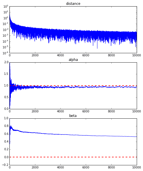
This seems to be due to the characteristics of the error function of the regression line this time, but as you can see from the graph below, for $ \ alpha $, the minimum curve is around $ \ alpha = 1 $. It has fallen around the value. However, since there are only very gradual changes in the vertical lines, it is difficult to get a gradient that causes vertical movement. If this is the usual steepest descent method, this curved surface itself does not change, so we aim for the minimum value gently along the valley, but in the first place, because this curved surface changes every time, it is in the $ \ beta $ direction. There seems to be no movement.

Now, did you have an image of stochastic gradient descent? I got an image by drawing this animation graph. The python code that draws the animation of this stochastic gradient descent method can be found at here, so try it if you like. Please try.

(Supplement) Find the parameters of the regression line by the maximum likelihood method

y_n = f(x_n, \alpha, \beta) + \epsilon_n　　　　(n =1,2,...,N)

That is, the error is

\epsilon_n = y_n - f(x_n, \alpha, \beta) 　　　　(n =1,2,...,N)  \\
\epsilon_n = y_n -\alpha x_n - \beta　　　　　　　　　　　　　　　　　　　

Can be represented by. If this error $ \ epsilon_i $ follows a normal distribution with mean = 0 and variance = $ \ sigma ^ 2 $, the likelihood of the error function is

L = \prod_{n=1}^{N} \frac{1}{\sqrt{2\pi\sigma^2}} \exp \left( -\frac{\epsilon_n^2}{2\sigma^2} \right)

And if you take the logarithm

\log L = -\frac{N}{2} \log (2\pi\sigma^2) -\frac{1}{2\sigma^2} \sum_{n=1}^{N} \epsilon_n^2

And if you retrieve only the terms that depend on the parameters $ \ alpha, beta $

l(\alpha, \beta) = \sum_{n=1}^{N} \epsilon_n^2 = \sum_{n=1}^{N} (y_n -\alpha x_n - \beta)^2

You can see that you should minimize. Use this as an error function

E({\bf w})=\sum_{n=1}^{N} E_n({\bf w}) = \sum_{n=1}^{N} (y_n -\alpha x_n - \beta)^2 \\
{\bf w} = (\alpha, \beta)^{\rm T}　　　　　　　　　　　　　　　　　　　　　　　

It is expressed as.