Implementation of particle filters in Python and application to state space models
There are various names such as particle filter / particle filter and sequential Monte Carlo (SMC), but in this article, we will use the name particle filter. I would like to implement this particle filter in Python and try to estimate the latent variables of the state space model.
The state space model is further divided into several models, but this time we will deal with the local model (first-order difference trend model), which is a simple model. If you want to know what else is in the trend type of this state space model, click here (http://www.statsmodels.org/stable/generated/statsmodels.tsa.statespace.structural.UnobservedComponents.html# Please refer to statsmodels.tsa.statespace.structural.UnobservedComponents).
\begin{aligned}
x_t &= x_{t-1} + v_t, \quad v_t \sim N(0, \alpha^2\sigma^2)\quad &\cdots\ {\rm System\ model} \\
y_t &= x_{t} + w_t, \quad w_t \sim N(0, \sigma^2)\quad &\cdots\ {\rm Observation\ model}
\end{aligned}
$ x_t $ represents the latent state at time t and $ y_t $ represents the observed value.
For the data to be used, use the sample data (http://daweb.ism.ac.jp/yosoku/) of "Basics of statistical modeling used for prediction".
 This test data can be obtained from here (http://daweb.ism.ac.jp/yosoku/).
Using the particle filter, you can estimate the latent state at each point in time using particles, that is, random numbers, as shown in the graph below. The red particles are particles, and you can filter by assigning weights based on likelihood to these particles and taking a weighted average, and you can estimate the latent state as shown by the green line. I will. As the observation model shows, the blue observation value (data that we have now) has noise that follows a normal distribution from this latent state, and [latent state value] + [ The model assumes that [noise] = [observed value as a realized value].

The algorithm for estimating the latent state value by filtering with this particle filter is explained below.
Click here for the flow animation.

1. Python code
The core ParticleFilter class is below.
The full code is here [https://github.com/matsuken92/Qiita_Contents/blob/master/particle_filter/particle_filter_class.ipynb)
class ParticleFilter(object):
    def __init__(self, y, n_particle, sigma_2, alpha_2):
        self.y = y
        self.n_particle = n_particle
        self.sigma_2 = sigma_2
        self.alpha_2 = alpha_2
        self.log_likelihood = -np.inf

    def norm_likelihood(self, y, x, s2):
        return (np.sqrt(2*np.pi*s2))**(-1) * np.exp(-(y-x)**2/(2*s2))

    def F_inv(self, w_cumsum, idx, u):
            if np.any(w_cumsum < u) == False:
                return 0
            k = np.max(idx[w_cumsum < u])
            return k+1

    def resampling(self, weights):
        w_cumsum = np.cumsum(weights)
        idx = np.asanyarray(range(self.n_particle))
        k_list = np.zeros(self.n_particle, dtype=np.int32) #List storage location of sampled k

        #Get subscripts to resample according to weight from uniform distribution
        for i, u in enumerate(rd.uniform(0, 1, size=self.n_particle)):
            k = self.F_inv(w_cumsum, idx, u)
            k_list[i] = k
        return k_list

    def resampling2(self, weights):
        """
Stratified sampling with low computational complexity
        """
        idx = np.asanyarray(range(self.n_particle))
        u0 = rd.uniform(0, 1/self.n_particle)
        u = [1/self.n_particle*i + u0 for i in range(self.n_particle)]
        w_cumsum = np.cumsum(weights)
        k = np.asanyarray([self.F_inv(w_cumsum, idx, val) for val in u])
        return k

    def simulate(self, seed=71):
        rd.seed(seed)

        #Number of time series data
        T = len(self.y)

        #Latent variable
        x = np.zeros((T+1, self.n_particle))
        x_resampled = np.zeros((T+1, self.n_particle))

        #Initial value of latent variable
        initial_x = rd.normal(0, 1, size=self.n_particle)   #--- (1)
        x_resampled[0] = initial_x
        x[0] = initial_x

        #weight
        w        = np.zeros((T, self.n_particle))
        w_normed = np.zeros((T, self.n_particle))

        l = np.zeros(T) #Likelihood by time

        for t in range(T):
            print("\r calculating... t={}".format(t), end="")
            for i in range(self.n_particle):
                #Apply 1st floor difference trend
                v = rd.normal(0, np.sqrt(self.alpha_2*self.sigma_2)) # System Noise #--- (2)
                x[t+1, i] = x_resampled[t, i] + v #Addition of system noise
                w[t, i] = self.norm_likelihood(self.y[t], x[t+1, i], self.sigma_2) # y[t]Likelihood of each particle with respect to
            w_normed[t] = w[t]/np.sum(w[t]) #Standardization
            l[t] = np.log(np.sum(w[t])) #Log-likelihood of each time

            # Resampling
            #k = self.resampling(w_normed[t]) #Particle subscripts obtained by re-sampling
            k = self.resampling2(w_normed[t]) #Particle subscripts acquired by re-sampling (layered sampling)
            x_resampled[t+1] = x[t+1, k]

        #Overall log-likelihood
        self.log_likelihood = np.sum(l) - T*np.log(n_particle)

        self.x = x
        self.x_resampled = x_resampled
        self.w = w
        self.w_normed = w_normed
        self.l = l

    def get_filtered_value(self):
        """
The value is calculated by filtering by the weighted average value by the weight of the likelihood.
        """
        return np.diag(np.dot(self.w_normed, self.x[1:].T))

    def draw_graph(self):
        #Graph drawing
        T = len(self.y)

        plt.figure(figsize=(16,8))
        plt.plot(range(T), self.y)
        plt.plot(self.get_filtered_value(), "g")

        for t in range(T):
            plt.scatter(np.ones(self.n_particle)*t, self.x[t], color="r", s=2, alpha=0.1)

        plt.title("sigma^2={0}, alpha^2={1}, log likelihood={2:.3f}".format(self.sigma_2,
                                                                                 self.alpha_2,
                                                                                 self.log_likelihood))
        plt.show()
2. How the particle filter works
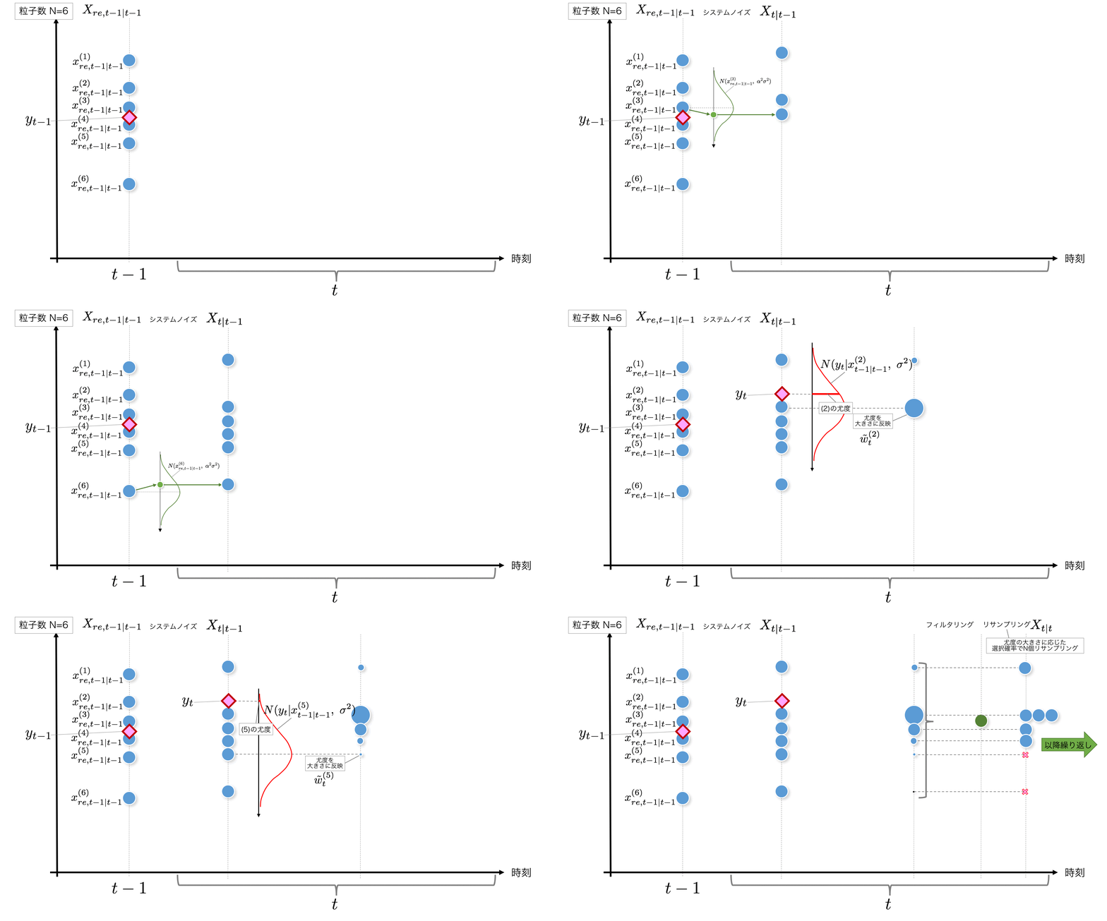
I will repost the animation of the process flow.

Below, I will explain one frame at a time.
STEP1:
It starts from t-1 point, but if t = 1, the initial value is required. Here, we will generate a random number that follows $ N (0, 1) $ as the initial value and use this as the initial value. If t> 1, the result of the previous time corresponds to this $ X_ {re, t-1 | t-1} $.

Here is the code for the initialization part of the particle.
initial_x = rd.normal(0, 1, size=self.n_particle) #--- (1)
STEP2: According to the system model, noise will be added when the current time $ t-1 $ is changed to the next time after $ t $. It is assumed here that it follows the normal distribution $ N (0, \ alpha ^ 2 \ sigma ^ 2) $. Do this for the number of particles.
x_t = x_{t-1} + v_t, \quad v_t \sim N(0, \alpha^2\sigma^2)\quad \cdots\ {\rm System\ model}

The code adds noise according to $ N (0, \ alpha ^ 2 \ sigma ^ 2) $ to each particle as shown below.
v = rd.normal(0, np.sqrt(self.alpha_2*self.sigma_2)) # System Noise #--- (2)
x[t+1, i] = x_resampled[t, i] + v #Addition of system noise
STEP3: After all the particle values $ x_ {t | t-1} $ after noise is obtained, $ y_t $, which is the observed value at time $ t $, is obtained, so the likelihood of each particle is calculated. To do. The likelihood calculated here is the most likely of the particle to the observed value $ y_t $ just obtained. I want to use this as the weight of the particle, so I put it in a variable and save it. This likelihood calculation is also performed for the number of particles.
Likelihood is
p(y_t|x_{t|t-1}^{(i)}) = w_{t}^{(i)} = {1 \over \sqrt{2\pi\sigma^2}} \exp \left\{
-{1 \over 2} {(y_t - x_{t|t-1}^{(i)})^2 \over \sigma^2}
\right\}
Calculate with. After calculating the likelihood for all particles, the normalized weights (to add up to 1)
\tilde{w}^{(i)}_t = { w^{(i)}_t \over \sum_{i=1}^N w^{(i)}_t}
Also prepare.

def norm_likelihood(self, y, x, s2):
    return (np.sqrt(2*np.pi*s2))**(-1) * np.exp(-(y-x)**2/(2*s2))

w[t, i] = self.norm_likelihood(self.y[t], x[t+1, i], self.sigma_2) # y[t]Likelihood of each particle with respect to
w_normed[t] = w[t]/np.sum(w[t]) #Standardization
STEP4: Weighted average using the weight $ \ tilde {w} ^ {(i)} _t $ saved earlier
\sum_{i=1}^N \tilde{w}^{(i)}_t x_{t|t-1}^{(i)}
Is calculated to be the filtered $ x $ value.

In the code, the following get_filtered_value () is applicable.
def get_filtered_value(self):
    """
The value is calculated by filtering by the weighted average value by the weight of the likelihood.
    """
    return np.diag(np.dot(self.w_normed, self.x[1:].T))
STEP5: Considering the weight $ \ tilde {w} ^ {(i)} _t $ based on the likelihood as the probability of being extracted,
X_{t|t-1}=\{x_{t|t-1}^{(i)}\}_{i=1}^N
Resample N pieces from. This is called resampling, but it is an image of an operation in which particles with low likelihood are eliminated and particles with high likelihood are split into multiple pieces.

k = self.resampling2(w_normed[t]) #Subscripts of particles acquired by resampling (layered sampling)
x_resampled[t+1] = x[t+1, k]
When resampling, create an empirical distribution function from $ \ tilde {w} ^ {(i)} _t $ as shown below, and create an inverse function to make the range of (0,1] uniform. Each particle can be extracted from a random number with a probability according to the weight.

F_inv () is the code that processes the inverse function, and resampling2 () is the code that performs layered sampling. Stratified sampling is implemented with reference to "Kalman Filter-Time Series Prediction and State Space Model Using R- (Statistics One Point 2)".
\begin{aligned}
u &\sim U(0, 1) \\
k_i &= F^{-1}((i-1+u)/N) \quad i=1,2,\cdots, N \\
x^{(i)}_{t|t} &= x^{(k_i)}_{t|t-1}
\end{aligned}
It's like that. Instead of generating N uniform random numbers between (0, 1], generate only one uniform random number between (0, 1 / N] and 1 / N between (0, 1] It is supposed to be staggered and sampling N pieces with an even width.

def F_inv(self, w_cumsum, idx, u):
        if np.any(w_cumsum < u) == False:
            return 0
        k = np.max(idx[w_cumsum < u])
        return k+1

def resampling2(self, weights):
    """
Stratified sampling with low computational complexity
    """
    idx = np.asanyarray(range(self.n_particle))
    u0 = rd.uniform(0, 1/self.n_particle)
    u = [1/self.n_particle*i + u0 for i in range(self.n_particle)]
    w_cumsum = np.cumsum(weights)
    k = np.asanyarray([self.F_inv(w_cumsum, idx, val) for val in u])
    return k
By performing this operation from t = 1 to T, particles can be generated and filtered.
The result is the graph below.

3. Verify that the implementation is correct by comparing it with the Kalman Filter results
Now, I want to check if the implemented particle filter behaves correctly, or if it outputs the same result by comparing it with the result of the Kalman filter in Stats Models just in case. I think
# Unobserved Components Modeling (via Kalman Filter)Execution of
import statsmodels.api as sm

# Fit a local level model
mod_ll = sm.tsa.UnobservedComponents(df.data.values, 'local level')
res_ll = mod_ll.fit()

print(res_ll.summary())

# Show a plot of the estimated level and trend component series
fig_ll = res_ll.plot_components(legend_loc="upper left", figsize=(12,8))
plt.tight_layout()

If you overlay this with the result of the particle filter, it fits almost perfectly! : laughing:

This is the implementation of the particle filter. The explanation of why this works is a must-read because Tomoyuki Higuchi (Author), the basics of statistical modeling used for prediction, is very easy to understand.
home work
- Add confidence interval at each point in time
- Forecast after T
- I haven't added fixed lug smoothing yet, so I want to add it.
- I want to think about hyperparameter search because it is not good at Grid Search.
- Supports trends other than local models and the addition of Seasonal terms
- Speeding up
reference
- Code used on this page https://github.com/matsuken92/Qiita_Contents/blob/master/particle_filter/particle_filter_class.ipynb
- Basics of statistical modeling used for prediction Tomoyuki Higuchi (Author) https://www.amazon.co.jp/dp/4061557955
- Kalman Filter-Time Series Prediction and State Space Model Using R- (Statistics One Point 2) Shunichi Nomura (Author) https://www.amazon.co.jp/dp/4320112539
- Computational Statistics 2 Markov Chain Monte Carlo Method and Surroundings (Frontier of Statistical Science 12) Yukito Iba (Author), Masaharu Tanemura (Author) https://www.amazon.co.jp/dp/4000068520
- StatsModels: Unobserved Components Modeling
http://www.statsmodels.org/stable/generated/statsmodels.tsa.statespace.structural.UnobservedComponents.html#statsmodels.tsa.statespace.structural.UnobservedComponents
Recommended Posts