[PYTHON] Learn Bayesian statistics from the basics to learn the M-H and HMC methods
Introduction (why did you choose this)
Sampling is one of the methods adopted in situations where integral calculation is difficult, but I have not understood the sampling method for a long time (for example, I do not understand PRML §11 ┐ (´ ー `) ┌ ). However, recently I sometimes read papers that use sampling methods, so I decided to study from the basics.
Recently, while being shaken by a train in the company slave business
Practical introduction to Bayesian statistics from the basics by Hamiltonian Monte Carlo method
Since I was reading the book, I would like to summarize the M-H sampling and HMC method that appear in Chapters 4 and 5. The contents are almost the same as the example in the book. I really wanted to go to Appendix B for slice sampling and NUTS, but my work exploded and I didn't have enough time (I'll do more later).
After organizing the following code, I will upload it to github or bitbucket.
example
The Poisson distribution is used as the probability distribution of rare events, and the gamma distribution is used as its prior distribution. Since the gamma distribution is a conjugate prior of the Poisson distribution, sampling is not necessary in the first place, but it is used as an example (§3 in this book).
Illustration of Poisson distribution
sample.py
import numpy as np
import scipy.stats as sst
import matplotlib.pyplot as plt
import seaborn as sns
%matplotlib inline

###Poisson distribution (mean 2.5)Example
from scipy.stats import poisson
mu = 2.5
x = np.arange(poisson.ppf(0.01, mu), poisson.ppf(0.99, mu))
plt.plot(x, poisson.pmf(x, mu), 'bo', ms=8, label='poisson pml')
plt.vlines(x, 0, poisson.pmf(x, mu), colors='b', lw=5, alpha=0.5)

Introduction of gamma distribution as prior distribution and calculation of posterior distribution
The posterior distribution is calculated assuming that the data (0, 1, 0, 0, 2, 0, 1, 0, 0, 1) that seems to be Poisson distribution is observed appropriately. As I wrote above, since it is a conjugate prior distribution in the first place, the shape of the posterior distribution can be understood.
sample.py
#data
x_data = np.array([0, 1, 0, 0, 2, 0, 1, 0, 0, 1])

#Prior distribution (mean 2 gamma distribution)
f_prev = gamma(a=6.0, scale=1.0/3.0)
x = np.linspace(0.0, 5.0, 100)
plt.plot(x, f_prev.pdf(x), 'b-', label='Prev')

#Ex-post distribution
n = x_data.shape[0]
ap = np.sum(x_data)
print("observe {0} positive {1}".format(n, ap))
f_post = gamma(a=6.0+ap, scale=1.0/(3.0 + n))
plt.plot(x, f_post.pdf(x), 'r--', label='Post')
plt.legend()

Sampling by Metropolis-Hastings method
Let the parameter be $ \ theta $. For the current value $ \ theta ^ {(t)} $ and the value $ \ theta_a $ sampled from the proposed distribution, it is probabilistically determined whether to demand $ \ theta_a
In the case of the Poisson distribution and the gamma distribution this time, the posterior distribution that we want to find is proportional to the product of the likelihood and the prior distribution (gamma distribution with parameters α = 11, λ = 13 in the example) according to Bayes' law, so $ r $ By transforming the formula of
sample.py
#data
x_data = np.array([0, 1, 0, 0, 2, 0, 1, 0, 0, 1])

#Likelihood
def log_likelihood(x, theta):
    x_probs = poisson.pmf(x, theta)
    return np.sum(np.log(x_probs))

#Gamma distribution kernel
def k_fg(theta, a, lbd): return np.exp(-lbd * theta) * (theta ** (a-1))

#Proposed distribution;Average theta,Standard deviation 0.Normal distribution of 5
def q(x, theta): return sst.norm.pdf(x, loc=theta, scale=0.5)

# M-H loop (initial value 1).0, 1000 times)
def metropolis_raw(N):
    current = 1.0 #initial value
    sample = []
    sample.append(current)

    for iter in range(N):
        a = sst.norm.rvs(loc=prop_m, scale=prop_sd)

        if a < 0: # reject (In the proposed distribution
            sample.append(sample[-1])
            continue

        T_next = q(current, a) * k_fg(a, a=11.0, lbd=13.0) * log_likelihood(x_data, a)
        T_prev = q(a, current) * k_fg(current, a=11.0, lbd=13.0) * log_likelihood(x_data, current)
        ratio = T_next / T_prev

        if ratio < 0: # reject
            sample.append(sample[-1])
        if ratio > 1 or ratio > sst.uniform.rvs():
            sample.append(a)
            current = a
        else:
            sample.append(sample[-1])

    return np.array(sample)

N = 10000
theta = metropolis_raw(N)
n_burn_in = 1000

# theta trace
plt.figure(figsize=(10, 3))
plt.xlim(0, len(theta)-n_burn_in)
plt.title("Trace plot from M-H sampling. burn-in:{}".format(n_burn_in))
plt.plot(theta[n_burn_in:], alpha=0.9, lw=.3)

# plot samples
plt.figure(figsize=(5,5))
plt.title("Histgram from M-H sampling.")
plt.hist(theta[n_burn_in:], bins=50, normed=True, histtype='stepfilled', alpha=0.2)
xx = np.linspace(0, 2.5,501)
plt.plot(xx, sst.gamma(11.0, 0.0, 1/13.).pdf(xx))
plt.show()
Is the implementation wrong, surprisingly not good


Independent M-H method
In the above example, the normal distribution (given parameters) was used as the proposed distribution, but isn't it okay if f and q are independent in the first place? → Independent M-H method
sample.py
import scipy.stats as sst

#Proposed distribution;normal distribution(Fixed parameters)
prop_m, prop_sd = 1.0, 0.5
def q(x): return sst.norm.pdf(x, loc=prop_m, scale=prop_sd)

#Replace the a and r calculations
a = sst.norm.rvs(loc=prop_m, scale=prop_sd)
r = (q(current)*k_fg(a,a=11.0, lbd=13.0)) / (q(a)*k_fg(current,a=11.0,lbd=13.0))


I'm worried about the implementation.
Random walk M-H method
Let's randomly walk the candidate points (straight ball) → If you use the normal distribution, put the proposed value (a) and variance so far in the mean appropriately.
sample.py
current = 4.0
list_theta = []
list_theta.append(current)

#For random walk (blur the given parameters on average)
def f_g(theta):
    prop_sd = np.sqrt(0.1)
    return sst.norm.rvs(loc=theta, scale=prop_sd)

###Replace the calculated part of a and r
a = f_g(current)
r = f_gamma(a) / f_gamma(current)


It will be a little better if you increase the number of repetitions.
Bonus (scipy function)
Sampling ability of the head family.
sample.py
import scipy.stats as sst
lbd = 1.0/13
plt.rcParams["figure.figsize"] = [4, 4]
a = 11.0
rv = sst.gamma(a, scale=lbd)
x = np.linspace(sst.gamma.ppf(0.01, a, scale=lbd), sst.gamma.ppf(0.99, a, scale=lbd), 100)
plt.plot(x, rv.pdf(x), 'r-', lw=5, alpha=0.6, label='gamma pdf')
plt.plot(x, rv.pdf(x), 'k-', lw=2, label='frozen pdf')
vals = rv.ppf([0.001, 0.5, 0.999])
np.allclose([0.001, 0.5, 0.999], sst.gamma.cdf(vals, a, scale=lbd))
r = sst.gamma.rvs(a, scale=lbd,size=9000)
plt.hist(r, normed=True, bins=100, histtype='stepfilled', alpha=0.2)
plt.legend(loc='best', frameon=False)

HMC method
I learned in high school physics that mechanical energy (kinetic energy + potential energy) is preserved when no external force is applied (no other loss due to light or heat). There should be many people. In analytical mechanics, we read this as Hamiltonian and discuss it in generalized coordinates. As a matter of fact (probably written earlier when you open a suitable book on analytical mechanics),
I will leave the details to the book, put the logarithmic posterior distribution as $ -h (\ theta) $, calculate the Hamiltonian as $ h (x) + \ frac {1} {2} p ^ 2 $, and follow the steps below. The HMC method is the method of sampling with (in the case of one dimension).
- [Leapfrog method](https://ja.wikipedia.org/wiki/%E3%83%AA%E3%83%BC%E3%83%97%E3%83%BB%E3%83%95 % E3% 83% AD% E3% 83% 83% E3% 82% B0% E6% B3% 95) Determine $ \ epsilon, L, T $ as parameters of.
- Determine the initial value $ \ theta ^ {(0)} $ and set $ i = 0 $ (repeat 3 to 6 until the specified $ i $)
- Sample from standard normal distribution… $ p ^ {(i)} \ sim \ mathcal {N} (p ^ {(i)} \ mid 0, 1) $
- Change $ \ theta ^ {(i)} $ and $ p ^ {(i)} $ by L steps by the Leapfrog method, and change the candidate points $ \ theta ^ {(a)}, p ^ {(a) } Calculate $
- $ r = \ exp \ (H (\ theta ^ {(t)}, p ^ {(t)}) --H (\ theta ^ {(a)}, p ^ {(a)}) ) As $, accept 5 assistant stores with probability $ \ min (1, r) $, and discard otherwise.
- t = t+1
Let's implement it and see how it works. Poisson distribution-Gamma distribution model with posterior distribution excluding normalization constants
hmc_sample.py
#Definition of the derivative of h and h
alpha, lbd = 11, 13
def _h(theta, alpha, lbd):
    return lbd * theta - (alpha - 1) * np.ma.log(theta)
def _hp(theta, alpha, lbd):
    return lbd - (alpha - 1) / theta
h = lambda theta: _h(theta, alpha, lbd)
hp = lambda theta: _hp(theta, alpha, lbd)

###Hamiltonian
def H(theta, p):
    return h(theta) + 0.5 * p * p

###Simple implementation of Leapfrog method
def lf(_th, _p, epsilon, L):
    l_p = [_p]
    l_th = [_th]
    for tau in range(1, L):
        p_t = l_p[-1]
        theta_t = l_th[-1]

        # 1/2
        p_t_half = p_t - 0.5 * epsilon * hp(theta_t)

        # update
        next_theta = theta_t + epsilon * p_t_half
        next_p = p_t_half - 0.5 * epsilon * hp(next_theta)

        # store
        l_p.append(next_p)
        l_th.append(next_theta)
    return (l_th[-1], l_p[-1])


###HMC sampling
N = 10000
moves = []
theta = [2.5]
p = []
L = 100
epsilon = 0.01

for itr in range(N):
    pv = sst.norm.rvs(loc=0, scale=1, size=1)[0]
    p.append(pv)

    # candidate by LF
    curr_th, curr_p = theta[itr], p[itr]
    cand_th, cand_p = lf(curr_th, curr_p, epsilon, L)

    # compute r by exp(H(curr) - H(cand))
    Hcurr = H(curr_th, curr_p)
    Hcand = H(cand_th, cand_p)
    r = np.exp(Hcurr - Hcand)
    # print("{0}\t{1:2.4f}\t{2:2.4f}".format(itr, cand_th, cand_p))
    # print("\t\t\t{0:2.3f}\t{1:2.3f}\t{2:2.3f}".format(Hcurr, Hcand, r))

    if r < 0:
        #reject
        theta.append(theta[-1])
        p.append(p[-1])
        continue
    if r >= 1 or r > sst.uniform.rvs():
        theta.append(cand_th)
        p.append(cand_p)

        moves.append( (curr_th, cand_th, curr_p, cand_p) )

        curr_th, curr_p = cand_th, cand_p
    else:
        #Reject
        theta.append(theta[-1])
Trace and histogram plots.


Good vibes.
Draw contour lines
hmc_sample.py
lin_p = np.linspace(-6.5, 6.5, 100.0)
lin_theta = np.linspace(0.01, 3.51, 100.0)
X, Y = np.meshgrid(lin_theta, lin_p)
Z = H(X, Y)
# 1dim h(theta)
xx = np.linspace(0.01, 3.01, 100)
plt.figure(figsize=(14, 7))
plt.title("h")
plt.plot(xx, h(xx), lw='1.5', alpha=0.8, color='r')
plt.xlim(-0.1, 3.5)
plt.xlabel("theta")
plt.ylabel("h(theta)")
# 2dim
plt.figure(figsize=(14,7))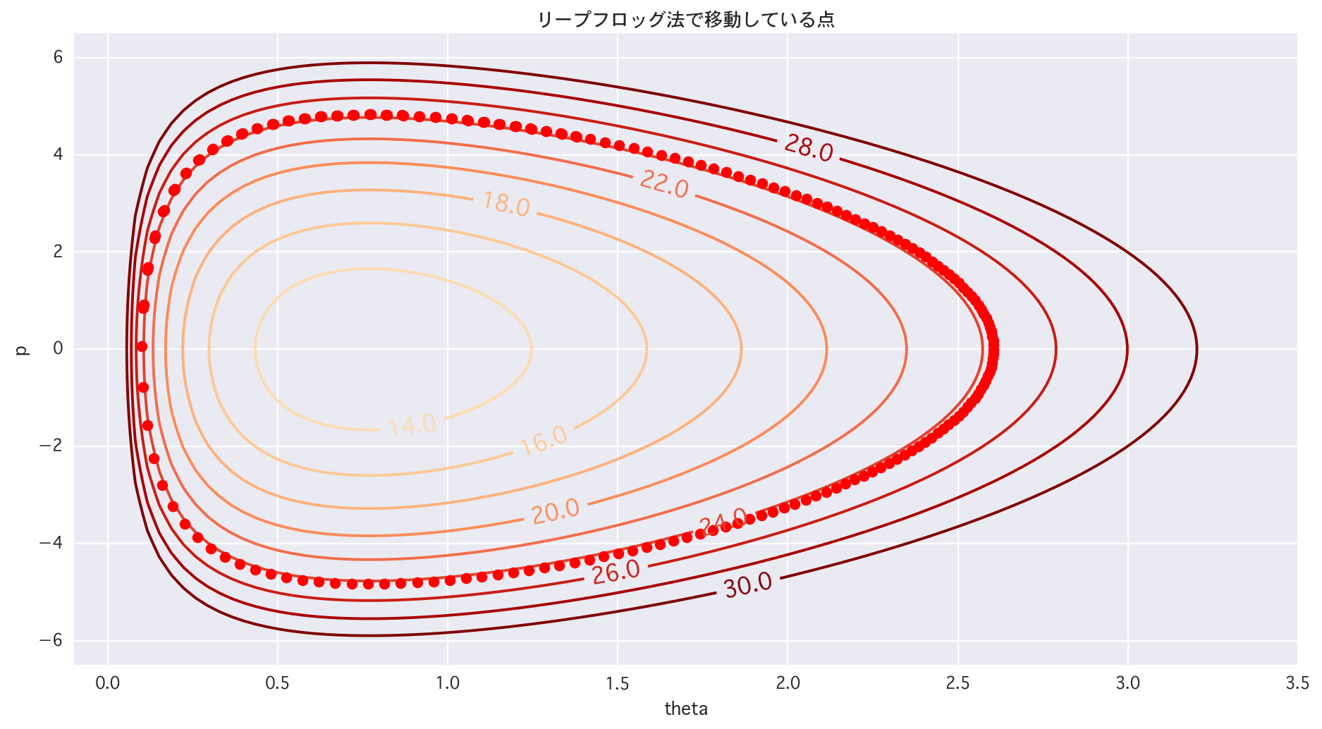
cont = plt.contour(X, Y, Z, levels=[i for i in range(10, 32, 2)], cmap="OrRd")
cont.clabel(fmt='%2.1f', fontsize=14)
plt.xlim(-0.1, 3.5); plt.ylim(-6.5, 6.5); plt.xlabel("theta"); plt.ylabel("p"); plt.show()


hmc_smaple.py
# 2dim (trace of LF)
# 1/4 areas
plt.figure(figsize=(14,7))
cont = plt.contour(X, Y, Z, levels=[i for i in range(10, 32, 2)], cmap="OrRd")
cont.clabel(fmt='%2.1f', fontsize=14)
for tau in range(1, len(p)):
    plt.plot(theta[tau], p[tau], 'ro')
plt.title(u"The point of moving by the Leapfrog method")
plt.xlim(-0.1, 3.5)
plt.ylim(-6.5, 6.5)
plt.xlabel("theta")
plt.ylabel("p")
plt.show()
Feel the desire to save Hamiltonian (appropriate)

hmc_sample.py
#From which point to which point
# 1/4 areas
plt.figure(figsize=(14,7))
cont = plt.contour(X, Y, Z, levels=[i for i in range(10, 32, 2)], cmap="OrRd")
cont.clabel(fmt='%2.1f', fontsize=14)
# for tau in range(1, len(p)):
#    plt.plot(theta[tau], p[tau], 'ro')
plt.title(u"The point of moving by the Leapfrog method")
plt.xlim(-0.1, 3.5)
plt.ylim(-6.5, 6.5)
plt.xlabel("theta")
plt.ylabel("p")

for i in range(len(moves)):
    t0, t1, p0, p1 = moves[i][0], moves[i][1], moves[i][2], moves[i][3]
    # plt.plot([t0, t1], [p0, p1], 'r-')
    plt.plot([t0, t1], [p0, p1], 'r-')
    plt.plot(t0, p0, 'ro')
    plt.plot(t1, p1, 'bo')

plt.show()

There is learning when you actually move it.
plans
What I left behind will be digested and updated later this year (flag)
- Slice Sampling
- NUTS
Recommended Posts