[PYTHON] Why is cross entropy used for the objective function of the classification problem?

What is a classification problem?

The classification problem classifies data into several categories and is one of the typical methods of machine learning.

Take a purchasing site as an example. Predict whether a user will buy or not buy a new product from a user's purchase information. Classification into two categories (classes) is called binary classification.

Classification predictions with more than two classes are called multiclass classification. Judgment of what is shown in the image (image recognition) is also one of the multi-class classification problems. It is also a classification problem to judge that it is a cat based on the image of a cat.

Cross entropy

Two probability distributions

P(x):Correct data distribution\\
Q(x):Predictive model distribution

In contrast, cross entropy is defined below.

L = - \sum_{x} P(x) \log{Q(x)}

The more similar the two probability distributions are, the smaller the cross entropy. Utilizing the properties of this function, it is often adopted as an objective function in machine learning (especially classification problems).

In this article, we will mathematically consider why cross entropy is often adopted for objective functions.

The following was helpful for a detailed explanation of cross entropy. http://cookie-box.hatenablog.com/entry/2017/05/07/121607

Binomial distribution (Bernoulli distribution)

In considering the classification problem, take the binomial distribution, which is the simplest probability distribution, as an example.

P(x_1) = p \;\;\; P(x_2) = 1 - p \\
Q(x_1) = q \;\;\; Q(x_2) = 1 - q \\

There are two colored balls, red and white, in the box, and the probability of drawing red is

P(Red) = p

The probability of drawing white

P(White) = 1 - p

It is easy to understand if you think about it. If you have a total of 10 balls, 2 red and 8 white

P(Red) = 0.2 \quad P(White) = 0.8

about it.

Now, at this time, the objective function is

\begin{align}
L &= - \sum_{x} P(x) \log{Q(x)} \\
  &= - p \log{q} - (1-p) \log{(1-q)}
\end{align}

Can be expanded.

Consider the following simple neural network. Imagine a scenario where you want to finally find the probability distribution $ q $. To give the previous example, I don't know the contents of the box at all, but I'm going to use some input data to build a probability distribution that draws a red ball as a model and predict the result.

y = \sum_{i} x_i w_i \\
\\
q(y) = \frac{1}{1+e^{-y}} :Sigmoid function

Here, $ x_i $ is input, $ w_i $ is weighted, $ y $ is an intermediate value, and $ q $ is output. The most typical sigmoid function is used as the activation function.

Neural network training

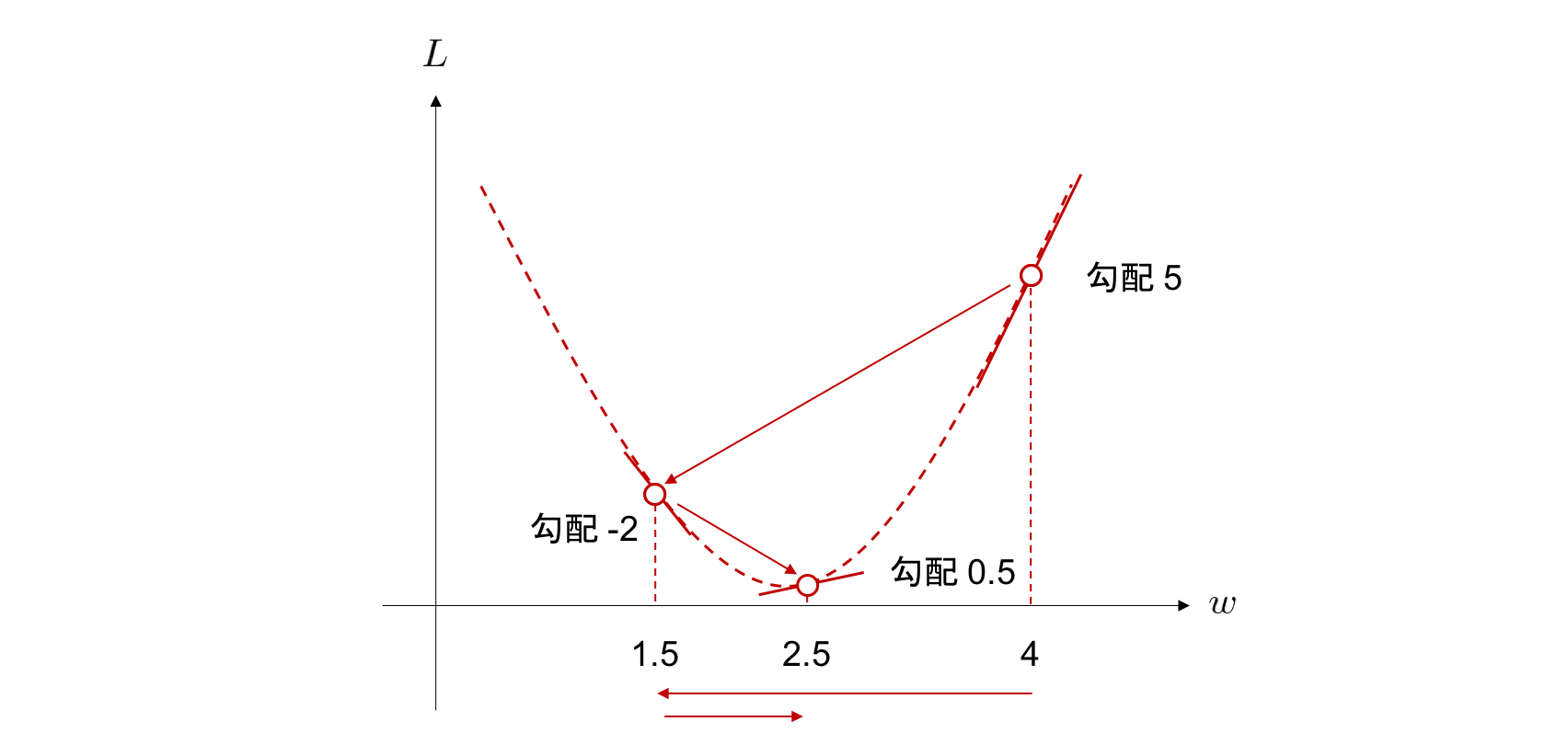
Train the neural network by finding the values of the parameters that minimize the value of the objective function. It uses one of the optimization algorithms, ** gradient descent **.

w \leftarrow w - \eta \frac{\partial L}{\partial w}

The gradient descent method is a method of repeatedly calculating ** learning rate x gradient of objective function ** to find the weight that takes the minimum value of the objective function.

The following Chainer Tutorial is very easy to understand for a detailed explanation of this area. https://tutorials.chainer.org/ja/13_Basics_of_Neural_Networks.html

Let's differentiate the objective function at once.

\frac{\partial L }{\partial w_i} = \frac{\partial y}{\partial w_i} \frac{\partial q }{\partial y}\frac{\partial L }{\partial q}

The first derivative is

\frac{\partial y}{\partial w_i} = \frac{\partial}{\partial w_i} \sum_i x_i w_i = x_i

The second derivative is

\begin{align}
\frac{\partial q }{\partial y} &= \frac{\partial}{\partial y} \frac{1}{1+e^{-y}} \\
&= \frac{\partial u}{\partial y}\frac{\partial}{\partial u} \frac{1}{u} \\
&= -e^{-y} (-u^{-2}) \\
&= \frac{e^{-y}}{1+e^{-y}}\frac{1}{1+e^{-y}} \\
&= \bigl( \frac{1+e^{-y}}{1+e^{-y}} - \frac{1}{1+e^{-y}} \bigr) \frac{1}{1+e^{-y}} \\
&= \bigl( 1-q(y) \bigr) q(y)
\end{align}

The third derivative is

\begin{align}
\frac{\partial L}{\partial q} &= \frac{\partial}{\partial q} \{ - p \log{q} - (1-p) \log{(1-q)} \} \\
&= - \frac{p}{q} + \frac{1-p}{1-q}

\end{align}

Because it can be calculated

\frac{\partial L }{\partial w_i} = x_i (1-q) q \bigl( - \frac{p}{q} + \frac{1-p}{1-q} \bigr) = x_i (q-p)

In other words

p = q

When is, the objective function takes the minimum value. In other words, this means that the distribution of the correct answer data and the distribution of the prediction model are exactly the same.

Well, I'm just saying the obvious thing. There are actually 8 reds and 2 whites in the box It predicts that red is 80% and white is 20%.

Apply to classification problems

Now, let's increase the variation a little more as a classification problem. For example, in a classification problem, categories can be represented by 0, 1.

Apple: [1, 0, 0]
Gorilla: [0, 1, 0]
Rappa: [0, 0, 1]

If it is a little more generalized

The correct answer for the class to which x belongs is

t=[t_1, t_2 …t_K]^T

Suppose it is given by the vector. However, suppose this vector is such that only one of $ t_k ; (k = 1,2,…, K) $ is 1, and the others are 0. This is called a one-hot vector.

Now that we can define the classification problem in this way, the objective function looks like this:

L = - \sum_x P(x) \log{ Q(x) } = - \log{ Q(x) }

$ Q (x) $ represents the probability that the training data will be the same as the teacher data. Let's plot it.

In the gradient descent method, the weight $ w_i $ that minimizes the objective function is obtained by repeatedly calculating ** learning rate × gradient of the objective function **. If the ** learning rate ** is extremely high, or if the ** objective function gradient ** is large, the learning efficiency seems to be good. It also reduces the number of calculation steps.

You can see that for $ 0 <Q (x) <1 $, the objective function $ L $ decreases sharply near $ Q (x) = 0 $. From this, if the teacher data and the learning result are too different, it can be interpreted that the amount of decrease per step is large. In the classification problem, if you select cross entropy as the objective function, the calculation efficiency is good.

It's easy to forget if you're actually using a library like Chainer or Pytorch. It's also good to look back on the basic theory so as not to forget it. I learned a lot.

reference https://mathwords.net/kousaentropy https://water2litter.net/rum/post/ai_loss_function/ http://yaju3d.hatenablog.jp/entry/2018/11/30/225841 https://avinton.com/academy/classification-regression/