[PYTHON] Chainer, RNN and machine translation

Natural language processing and neural networks

In the last few years, neural networks have become very popular in the field of natural language processing as well.

Natural language processing mainly analyzes word arrays and syntax trees, and models based on recurrent neural networks [^ 1] and recursive neural networks [^ 1] to express these contained information. Is frequently used. The biggest feature of these is that ** neural networks have some kind of data structure **, and although there are not so many nodes per layer, the network connection is complicated, and each data input It has the characteristic that the shape of the network itself changes. For this reason, there was a problem that it was difficult to build with a toolkit that assumed the traditional feedforward neural network.

Chainer is a powerful neural network framework that generally solves such problems. It can be used if you know the Python grammar and a little NumPy, and the calculation formula on the source code is automatically stored as the connection information of the neural network, so ** If you parse the input data, it will be automatically There is a ~~ cheat-like ~~ feature called ** that can be analyzed with a neural network.

The Chainer sample collection that I recently wrote down also implements language models, word dividers, translation models, etc., but all of them are basic parts (in the code). The forward function) can be implemented in half a day, or an hour if it is short. As you can see from the sample, it's more like spending most of your effort on peripheral code that organizes your data.

In this article, we will mainly explain how to implement recurrent neural networks in Chainer and the encoder-decoder translation model, which is an application in natural language processing.

• The content of the article is based on Chainer 1.4 or earlier. We will support the 1.5 series by watching the situation. *

Recurrent Neural Network

The most basic recurrent neural network (RNN) is an orthodox three-layer neural network with hidden layer feedback, as shown in the following figure.

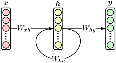
Although it is a simple model, the translation model introduced later is made by combining RNNs. In addition, RNN alone is an excellent product that can easily surpass the conventional * N * -gram model when used in a language model. [^ 2]

If you write down the above figure in the formula,

\begin{align}
{\bf h}_n & = \tanh \bigl( W_{xh} \cdot {\bf x}_n + W_{hh} \cdot {\bf h}_{n-1} \bigr), \\
{\bf y}_n & = {\rm softmax} \bigl( W_{hy} \cdot {\bf h}_n \bigr)
\end{align}

And use this as it is as a calculation formula on Chainer.

For now, let's consider an RNN language model that "enters a word ID and predicts the next word ID". [^ 3] First, define the ** model **. A model is a ** set of learnable parameters **, and $ W_ {\ * \ *} $ in the above figure corresponds to this. In this case, $ W_ {\ * \ *} $ are all linear operators (matrix), so use Linear or ʻEmbedID in chainer.functions. ʻEmbedID is Linear when the input side is a one-hot vector, and you can pass the ID of the firing element instead of the vector.

from chainer import FunctionSet
from chainer.functions import *

model = FunctionSet(
  w_xh = EmbedID(VOCAB_SIZE, HIDDEN_SIZE), #Input layer(one-hot) ->Hidden layer
  w_hh = Linear(HIDDEN_SIZE, HIDDEN_SIZE), #Hidden layer->Hidden layer
  w_hy = Linear(HIDDEN_SIZE, VOCAB_SIZE), #Hidden layer->Output layer
)  

VOCAB_SIZE represents the number of word types and HIDDEN_SIZE represents the dimension of the hidden layer.

Next, define a forward function that does the actual parsing. Here, basically, the network structure in the above figure is reproduced according to the model definition and the actual input data, and the final desired value is calculated. In the case of the language model, the ** sentence combination probability ** expressed in the following formula is calculated.

\begin{align}
\log {\rm Pr} \bigl( {\bf w} \bigr) & = \sum_{n=1}^{|{\bf w}|} \log {\rm Pr} \bigl( w_n \ \big| \ w_1, w_2, \cdots, w_{n-1} \bigr) \\
& = \sum_{n=1}^{|{\bf w}|} \log {\bf y}_n\big[ {\rm index} \bigl( w_n \bigr) \big]
\end{align}

The following is a code example, but since Chainer is premised on mini-batch processing, the data dimension is increased by one (batch processing is not performed in the code).

import math
import numpy as np
from chainer import Variable
from chainer.functions import *

def forward(sentence, model): #sentence is an array of str. Assuming output such as MeCab.
  sentence = [convert_to_your_word_id(word) for word in sentence] #Convert words to IDs. Implement it yourself.
  h = Variable(np.zeros((1, HIDDEN_SIZE), dtype=np.float32)) #Initial value of hidden layer
  log_joint_prob = float(0) #Sentence join probability

  for word in sentence:
    x = Variable(np.array([[word]], dtype=np.int32)) #Next input layer
    y = softmax(model.w_hy(h)) #Probability distribution of the next word
    log_joint_prob += math.log(y.data[0][word]) #Update of join probability
    h = tanh(model.w_xh(x) + model.w_hh(h)) #Hidden layer update

  return log_joint_prob #Returns the calculation result of the join probability

Now you can find the probability of the sentence. However, the above does not include the calculation of the loss function to train the model. Since the softmax function is used in the final stage this time, use chainer.functions.softmax_cross_entropy to find the cross entropy with the correct answer and use it as the loss function.

def forward(sentence, model):
  ...

  accum_loss = Variable(np.zeros((), dtype=np.float32)) #Initial value of cumulative loss
  ...

  for word in sentence:
    x = Variable(np.array([[word]], dtype=np.int32)) #Next input layer(=This correct answer)
    u = model.w_hy(h)
    accum_loss += softmax_cross_entropy(u, x) #Accumulation of loss
    y = softmax(u)
    ...

  return log_joint_prob, accum_loss #Cumulative loss is also returned

Now you can study.

from chainer.optimizers import *
...

def train(sentence_set, model):
  opt = SGD() #Use stochastic gradient descent
  opt.setup(model) #Initialization of learner
  for sentence in sentence_set:
    opt.zero_grad(); #Gradient initialization
    log_joint_prob, accum_loss = forward(sentence, model) #Loss calculation
    accum_loss.backward() #Backpropagation of error
    opt.clip_grads(10) #Suppress too large gradient
    opt.update() #Parameter update

Basically, this is the only Chainer process. In the past, I used to write a program with an unpleasant number of lines for such a neural network, but Chainer has almost all the troublesome calculations hidden in the Python syntax, so such a short description is written. It will be possible. As long as you remember how to use Chainer, you can quickly write and try out the recently proposed model or the original model you just came up with. [^ 4]

Encoder-decoder translation model

As a slightly complicated example of applying RNN, let's implement ** encoder-decoder translation model **, which is a machine translation method using neural networks. This is a translation model in which all processes from input to output are described by a neural network, and despite its simplicity, it achieves accuracy comparable to that of conventional translation models, which surprised researchers at the time of presentation. Was welcomed.

There are various variants of the Encoder-decoder translation model, but here I will write the model shown below, which is also implemented in my sample collection.

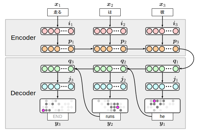
The idea is simple: two RNNs, one on the input language side (encoder) and one on the output language side (decoder), are prepared and connected by an intermediate node. The interesting thing about this model is that the output side generates a terminal symbol along with the word, so ** the model itself decides the end of the translation **. However, conversely, if learning of this terminal symbol fails, words will be generated infinitely, so if the process does not end even if an appropriate number of words are actually generated, it is necessary to discontinue the process. there is.

$ {\ bf i} $ and $ {\ bf j} $ are called ** embedding layers ** and represent compressed word information in dimensions. Also, the input word string is inverted, but it has been found that this method gives good translation results experimentally. The reason is not very clear, but it is interpreted as because the encoder and decoder are in a conversion / inverse relationship.

I will write the code immediately, but first let's put it in the calculation formula. It looks like this:

\begin{align}
{\bf i}_n & = \tanh \bigl( W_{xi} \cdot {\bf x}_n \bigr), \\
{\bf p}_n & = {\rm LSTM} \bigl( W_{ip} \cdot {\bf i}_n + W_{pp} \cdot {\bf p}_{n-1} \bigr), \\
{\bf q}_1 & = {\rm LSTM} \bigl( W_{pq} \cdot {\bf p}_{|{\bf w}|} \bigr), \\
{\bf q}_m & = {\rm LSTM} \bigl( W_{yq} \cdot {\bf y}_{m-1} + W_{qq} \cdot {\bf q}_{m-1} \bigr), \\
{\bf j}_m & = \tanh \bigl( W_{qj} \cdot {\bf q}_m \bigr), \\
{\bf y}_m & = {\rm softmax} \bigl( W_{jy} \cdot {\bf j}_m \bigr).
\end{align}

Here we are using LSTMs for the transition between hidden layers $ {\ bf p} $ and $ {\ bf q} $. [^ 5] can be understood by looking at the figure, but since the encoder side is located far from the position $ {\ bf y} $ where the loss is actually calculated, the normal activation function can be used. This is because there is a problem that it cannot be learned well. Such a model requires pre-learning of weights or an element that can store long-distance dependencies such as LSTM.

By the way, if you look at the above figure and formula, you can see that there are 8 types of transition $ W_ {\ * \ *} $. These are the parameters we will learn this time, and we will list them in the model definition.

model = FunctionSet(
  w_xi = EmbedID(SRC_VOCAB_SIZE, SRC_EMBED_SIZE), #Input layer(one-hot) ->Input embed layer
  w_ip = Linear(SRC_EMBED_SIZE, 4 * HIDDEN_SIZE), #Input embed layer->Input hidden layer
  w_pp = Linear(HIDDEN_SIZE, 4 * HIDDEN_SIZE), #Input hidden layer->Input hidden layer
  w_pq = Linear(HIDDEN_SIZE, 4 * HIDDEN_SIZE), #Input hidden layer->Output hidden layer
  w_yq = EmbedID(TRG_VOCAB_SIZE, 4 * HIDDEN_SIZE), #Output layer(one-hot) ->Output hidden layer
  w_qq = Linear(HIDDEN_SIZE, 4 * HIDDEN_SIZE), #Output hidden layer->Output hidden layer
  w_qj = Linear(HIDDEN_SIZE, TRG_EMBED_SIZE), #Output hidden layer->Output embedding layer
  w_jy = Linear(TRG_EMBED_SIZE, TRG_VOCAB_SIZE), #Output hidden layer->Output hidden layer
)  

It is necessary to pay attention to the $ W_ {ip}, W_ {pp}, W_ {pq}, W_ {yq}, W_ {qq} $ parameters that are input to the LSTM. You need to multiply the dimension by a factor of four. The LSTM implemented by Chainer has three types of inputs, input gate, output gate, and forget gate, in addition to normal inputs, and such an implementation is required to combine these as one vector. I have. [^ 6]

Next, write the forward function. Note that LSTMs have an internal state, so we need another Variable when calculating $ {\ bf p} $ and $ {\ bf q} $.

# src_sentence:The word string you want to translate e.g. ['he', 'Is', 'Run']
# trg_sentence:Word string representing the translation of the correct answer e.g. ['he', 'runs']
# training:Learning or prediction? Affects the behavior of the decoder.
def forward(src_sentence, trg_sentence, model, training):

  #Conversion to word ID (implement appropriately by yourself)
  #Add a terminal symbol to the correct translation.
  src_sentence = [convert_to_your_src_id(word) for word in src_sentence]
  trg_sentence = [convert_to_your_trg_id(word) for wprd in trg_sentence] + [END_OF_SENTENCE]

  #Initial value of LSTM internal state
  c = Variable(np.zeros((1, HIDDEN_SIZE), dtype=np.float32))

  #Encoder
  for word in reversed(src_sentence):
    x = Variable(np.array([[word]], dtype=np.int32))
    i = tanh(model.w_xi(x))
    c, p = lstm(c, model.w_ip(i) + model.w_pp(p))

  #Encoder->decoder
  c, q = lstm(c, model.w_pq(p))

  #decoder
  if training:
    #When learning, use the correct translation as y and return the cumulative loss as a result of forward.
    accum_loss = np.zeros((), dtype=np.float32)
    for word in trg_sentence:
      j = tanh(model.w_qj(q))
      y = model.w_jy(j)
      t = Variable(np.array([[word]], dtype=np.int32))
      accum_loss += softmax_cross_entropy(y, t)
      c, q = lstm(c, model.w_yq(t), model.w_qq(q))
    return accum_loss
  else:
    #At the time of prediction, y generated by the translator is used for the next input, and the word string generated as a result of forward is returned.
    #Select the word with the highest probability in y, but you don't need to take softmax.
    hyp_sentence = []
    while len(hyp_sentence) < 100: #Do not generate more than 100 words
      j = tanh(model.w_qj(q))
      y = model.w_jy(j)
      word = y.data.argmax(1)[0]
      if word == END_OF_SENTENCE:
        break #Finished because the terminal symbol was generated
      hyp_sentence.append(convert_to_your_trg_str(word))
      c, q = lstm(c, model.w_yq(y), model.w_qq(q))
    return hyp_sentence

It's a bit long, but if you read it carefully, you'll see that the arrows in the figure above correspond to each part of the code. After that, if you add a learner similar to RNN outside this code, it will be fine and you will be able to learn your own translation data.

Now, how this model learns, let's learn using the sample data of Japanese-English translation placed in here. If you study about 10,000 sentences with 2000 vocabulary, 100 embedded layer, and 100 hidden layer, you will get the following translation results for each generation (I used the program of the sample collection for learning). 2017/7/21: The link of the sample data has been re-linked. </ font>

input:How was your vacation?
output:
1: the is is a of of <unk> .
2: the 't is a <unk> of <unk> .
3: it is a good of the <unk> .
4: how is the <unk> to be ?
5: how do you have a <unk> ?
6: how do you have a <unk> ?
7: how did you like the <unk> ?
8: how did you like the weather ?
9: how did you like the weather ?
10: how did you like your work ?
11: how did you like your vacation ?
12: how did you like your vacation ?
13: how did you the weather to drink ?
14: how did you like your vacation ?
15: how did you like your vacation ?
16: how did you like your vacation ?
17: how did you like your vacation ?
18: how did you like your vacation ?
19: how did you enjoy your vacation ?
20: how did you enjoy your vacation now ?
21: how did you enjoy your vacation for you ?
22: how did you enjoy your vacation ?

input:She looks happy.
output:
1: she is a of of of .
2: she is a good of of .
3: she is a good of <unk> .
4: she is a good of <unk> .
5: she is a good of <unk> .
6: she is a good of his morning .
7: she is a good of his morning .
8: she is a good of his morning .
9: she is a good of his morning .
11: she is a good of his morning .
12: she is a good of his morning .
13: she is a good of his morning .
14: she is a good of his morning .
15: she is a good at tennis .
16: she is a good at tennis .
17: she is a good at tennis .
18: she is a good of the time .
19: she seems to be very very happy .
20: she is going to be a student .
21: she seems to be very very happy .
22: she seems to be very very happy .
23: she seems to be very happy .

input:I feel cold this morning.
output:
1: i 'm a of of of .
2: i 'm a <unk> of the <unk> .
3: it is a good of <unk> .
4: it is a good of <unk> .
5: it is a good of <unk> .
6: it is a good of the day .
7: it 's a good of <unk> .
8: it 's a good of <unk> .
9: it 's a good of <unk> .
10: it 's a good of <unk> today .
11: i 'm a good <unk> of time .
12: i 'm a good <unk> of time .
13: i 'm a good <unk> of time .
14: i 'm very busy this <unk> today .
15: i 'm very busy this morning time .
16: i 'm very busy this morning time .
17: i 'm very busy this time .
18: i 'm very busy this time .
19: i have a lot of cold here .
20: i have a lot of <unk> here .
21: i have a lot of <unk> time .
22: i 'm very busy this morning time .
23: i have a lot of cold here .
24: i have a lot of cold here .
25: i have a lot of that morning .
26: i have a lot of cold here .
27: i have a lot of cold here .
28: i have a cold , will do .
29: i feel cold this morning this morning .