[PYTHON] Time series analysis part 4 VAR
1. Overview
- Following Part 3 (https://qiita.com/asys/items/9d40172e72dd01caa293), I am studying based on "Measurement time series analysis of economic and financial data".
- This time, about the part corresponding to Chapter 4, the VAR model.
2. What is a VAR model?
- The VAR model is an extension of the AR model multivariate.
VAR(p) : \mathbb{y}_t=\mathbb{c}+ \Phi _1 \mathbb{y} _{t-1} + \cdots + \Phi _1 \mathbb{y} _{t-p} + \epsilon _t, \quad \epsilon _t \sim W.N.(\Sigma) - As you can see from the formula, it is characterized in that it does not contain other variables at the same time.
*The constant condition is that the absolute values of all the solutions of the following AR characteristic equations are greater than 1.
|\mathbb{I} _n - \Phi _1 z - \cdots - \Phi _p z^p|=0
However,\mathbb{I} _n Isn\times n Is the identity matrix of. - For model estimation, each equation may be estimated individually by OLS, and it can be estimated by the same method as AR model estimation.
3. Granger causality
Definition
- Granger causality was devised so that the presence or absence of causality can be determined only from the data regarding the causal relationship between variables.
- For $ \ mathbb {x} _t $, the set of information available at time $ t $ is $ \ Omega _t $, $ \ Omega _t $ minus $ \ mathbb {y} _t $ is $ \ Let's say tilde {\ Omega} _t $. When the MSE based on $ \ Omega _t $ is smaller than the MSE for the prediction of future $ \ mathbb {x} $ based on $ \ tilde {\ Omega} _t $, $ \ mathbb {y} _t $ There is a Granger causality from to $ \ mathbb {x} _t $.
- In other words, there is causality when the information of $ \ mathbb {y} _t $ improves the prediction accuracy in predicting $ \ mathbb {x} _t $.
- Granger causality is a necessary condition for the existence of causality in the usual sense, but it is not a sufficient condition.
Test
- Let $ SSR _1 $ be the estimated residual sum of squares using $ \ Omega _t $, and $ SSR _0 $ be the estimated residual sum of squared using $ \ tilde {\ Omega} _t $.
- Calculate the $ F $ statistic as follows: However, $ r $ is the number of constraints required for the test.
$ F \ equiv \ frac {\ frac {(SSR_0-SSR_1)} {r}} {\ frac {SSR_1} {(T-np-1)}} $ - $ rF $ is known to asymptotically follow $ \ chi ^ 2 (r) $, which is used to determine Granger causality.
Analysis example
data
- The data used was a dataset called FI2010. From here You can download it by clicking Access this dataset freely. Under Data Availability.
- Although details are omitted here, it is a data set of board information on stock exchanges. I used it to get used to it because it is a dataset that I personally want to touch in the future.
- Here, we analyze the degree of imbalance between the stock price transition (hereinafter referred to as the rate of change in the medium price) and the best quote quantity. Regarding the best quote quantity at a certain point, if there are more BIDs, it is thought that there are more buyers than sellers, and it is speculated that this may lead to a future rise in stock prices.
Preprocessing
#Read data.
data = pd.read_csv('Train_Dst_Auction_DecPre_CF_1.txt', header=None, delim_whitespace=True)
#The first 4 lines are the best ASK/It is the price and quantity data for BID.
#In addition, the first 3900 columns are the data for the first issue.
pr = data.iloc[:4,:3900].T
pr.columns = ['ask_p','ask_v','bid_p','bid_v']
#Calculate the medium price from the best ASK and best BID.
pr['mid_p'] = (pr['ask_p'] + pr['bid_p']) / 2
#Calculate the rate of change of the medium price.
pr['p_chg'] = pr['mid_p'].pct_change()
#Calculate the degree of imbalance between the quantities of ASK and BID.
pr['v_imb'] = (pr['ask_v'] / pr['bid_v']).apply(np.log)
pr = pr.dropna()
-
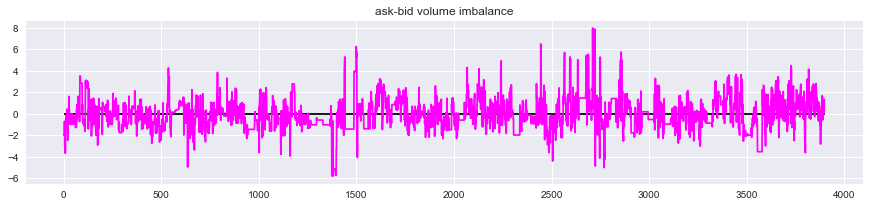
The plot of the data to be used is as follows.

-
The degree of imbalance in the best quote quantity is calculated as
$ \ qquad Imbalance = \ ln \ frac {V_ {ask}} {V_ {bid}} $
, and the value is positive. In the case of, the selling quantity is larger, and when the value is negative, the buying quantity is larger. -
If the value of the degree of imbalance is positive and the selling quantity is larger at the previous point, it is easy to check whether the stock price is falling at the moment.
#Cases where there are more sellers at the previous time
print('sell > buy ', pr.loc[pr['v_imb'].shift(-1)>1, 'p_chg'].sum())
#Cases where there are more buyers at the previous time
print('sell < buy ', pr.loc[pr['v_imb'].shift(-1)<1, 'p_chg'].sum())
# sell > buy  -0.0060484707428217765
# sell < buy  0.027729879129729684
On average, if there are many sells, the medium price is falling, and if there are many buys, the medium price is rising.
Granger causality test
- Use the familiar stats models every time.
#First, load the library and feed the data.
from statsmodels.tsa.vector_ar.var_model import VAR
model = VAR(pr[['v_imb','p_chg']].values)
- Next, determine the order of the model. This is the value corresponding to p in VAR (p). This is also one shot if you use the library.
model.select_order(10).summary()
| AIC | BIC | FPE | HQIC | |
|---|---|---|---|---|
| 0 | -15.49 | -15.48 | 1.880e-07 | -15.49 |
| 1 | -16.29 | -16.28 | 8.405e-08 | -16.29 |
| 2 | -16.31 | -16.30 | 8.217e-08 | -16.31 |
| 3 | -16.32 | -16.30 | 8.173e-08 | -16.31 |
| 4 | -16.33* | -16.30* | 8.101e-08* | -16.32* |
| 5 | -16.33 | -16.29 | 8.103e-08 | -16.32 |
| 6 | -16.33 | -16.29 | 8.108e-08 | -16.31 |
| 7 | -16.33 | -16.28 | 8.112e-08 | -16.31 |
| 8 | -16.33 | -16.27 | 8.116e-08 | -16.31 |
| 9 | -16.33 | -16.27 | 8.111e-08 | -16.31 |
| 10 | -16.33 | -16.26 | 8.120e-08 | -16.30 |
- For the time being, when looking at the order up to 10, it was said that $ p = 4 $ was good for all of the four default criteria, so the order is decided to be 4.
- Next, let's look at Granger causality.
#Create a model with an order of 4.
var_model = model.fit(4)
#Granger causality test. causing causing=0('v_imb')From used=1('p_chg')Test causality to.
Granger = var_model.test_causality(causing=0, caused=1)
Granger.summary()
| Test statistic | Critical value | p-value | df |
|---|---|---|---|
| 9.531 | 2.373 | 0.000 | (4, 7772) |
- Looking at the p-value, it is smaller than 0.05, so it can be said that Granger causality exists. After all, the degree of imbalance of the board seems to affect the subsequent transition of stock prices.
- By the way, on the contrary, the causality from the stock price transition to the degree of imbalance of the board was tested as follows.
Granger = var_model.test_causality(causing=1, caused=0)
Granger.summary()
| Test statistic | Critical value | p-value | df |
|---|---|---|---|
| 0.9424 | 2.373 | 0.438 | (4, 7772) |
- Here, the P value was larger than 0.05, and the result was that no causality was observed. It seems that there is a relationship such as an increase in the number of items for sale due to the rise in stock prices, but the Granger causality did not exist, probably because the time span being analyzed was too short.
4. Impulse Response Function
Non-orthogonalized impulse response function
- In a general VAR model, the change of $ y_ {i, t + k} $ after k period when a shock of 1 unit is given to the perturbation term $ \ epsilon_ {jt} $ of $ y_ {jt} $. As a function.
IRF_{ij}(k)=\frac{\partial y_{i,t+k}}{\partial \epsilon_{jt}} - It is assumed that there is no correlation between the disturbance terms, but in reality there are many cases where there is a correlation between $ \ epsilon_ {it} $ and $ \ epsilon_ {jt} $. The problem is that it has not been modeled well.
Orthogonalized impulse response function
- Dispersion of disturbance terms Impulse function when the covariance matrix is triangulated, decomposed into disturbance terms that are uncorrelated with each other, and then a shock of 1 unit is given to the disturbance terms.
- In a typical VAR model,
$ \ qquad VAR (p): \ mathbb {y} _t = \ mathbb {c} + \ Phi _1 \ mathbb {y} _ {t-1} + \ cdots + \ Phi _1 \ mathbb {y} _ {tp} + \ epsilon _t, \ quad \ epsilon _t \ sim WN (\ Sigma) $
$ A $ is a lower triangular matrix whose diagonal component is equal to 1, $ D Using $ as a diagonal matrix, it is triangulated as
$ \ qquad \ Sigma = ADA'$
, and
$ \ qquad u \ _ t = A ^ {-1} \ epsilon \ _t $
You can get the orthogonal disturbance term $ u \ _t $ in the form>. IRF_{ij}(k)=\frac{\partial y_{i,j+k}}{\partial u_{jt}} - Due to the use of triangulation, $ \ epsilon_ {kt} $ is a linear sum of $ u_ {1t}, \ cdots, u_ {kt} $. Therefore, the order of the variables affects the result.
Analysis example
- We will continue to use the board data used for Granger causality.
#Create a model with an order of 4.
var_model = model.fit(4)
# k=Calculate impulse responses up to 10.
IRF = var_model.irf(10)
#Plot the results. orth=False means non-orthogonalization.
IRF.plot(orth=False)
plt.show()
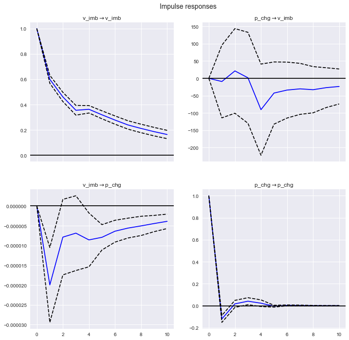
- What we want to pay attention to is the impulse response of v_imb → p_chg at the bottom left. A negative reaction appears after one period, and then the reaction gradually decreases. An increase in the degree of imbalance by one unit means more sales, suggesting a subsequent decline in stock price performance.
5. ANOVA
Definition
- The ratio of the orthogonal disturbance term $ u_ {j, t + 1}, \ cdots, u_ {j, t + k} $ of $ y_j $ to the MSE of the k-period prediction of $ y_i
. It is called the relative variance contribution rate (RVC). *About the n-variable VAR model y_iThe MSE for the k-term forecast is \mathbb{u}_{t+1},\cdots,\mathbb{u}_{t+k}Because it is a linear sum of \qquad \hat{e}_{i,t+k|t}=\sum_{h=1}^{k}w_{1,t+h}^{i}u_{1,t+h}+\cdots+\sum_{h=1}^{k}w_{n,t+h}^{i}u_{n,t+h}
Then\qquad where \quad \sigma\_l^2=E(u\_{lt}^2)
With\qquad RVC\_{ij}(k)=\frac{\sigma\_j^2\sum\_{h=1}^{k}(w\_{j,t+h}^i)^2}{\sum\_{l=1}^{n}\sigma\_l^2\sum\_{h=1}^{k}(w\_{l,t+h}^i)^2}
It can be expressed as.
Analysis example
- Continue to use FI2010 board data.
#Create a model with an order of 4.
var_model = model.fit(4)
# k=Calculate the variance contribution ratio up to 10.
FEVD = var_model.fevd(10)
#Plot the results.
FEVD.plot()
plt.show()
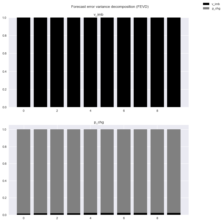
- This is too difficult to understand, so let's look at specific numbers.
FEVD.summary()
| FEVD for v_imb | v_imb | p_chg |
|---|---|---|
| 0 | 1.000000 | 0.000000 |
| 1 | 0.999994 | 0.000006 |
| 2 | 0.999969 | 0.000031 |
| 3 | 0.999971 | 0.000029 |
| 4 | 0.999572 | 0.000428 |
| 5 | 0.999511 | 0.000489 |
| 6 | 0.999478 | 0.000522 |
| 7 | 0.999452 | 0.000548 |
| 8 | 0.999418 | 0.000582 |
| 9 | 0.999397 | 0.000603 |
| FEVD for p_chg | v_imb | p_chg |
|---|---|---|
| 0 | 0.012342 | 0.987658 |
| 1 | 0.018310 | 0.981690 |
| 2 | 0.018871 | 0.981129 |
| 3 | 0.019158 | 0.980842 |
| 4 | 0.019791 | 0.980209 |
| 5 | 0.020477 | 0.979523 |
| 6 | 0.020889 | 0.979111 |
| 7 | 0.021208 | 0.978792 |
| 8 | 0.021472 | 0.978528 |
| 9 | 0.021678 | 0.978322 |
- It can be seen that the contribution of p_chg to the variance of v_imb is very low, which is consistent in terms of Granger causality and impulse response.
- On the contrary, v_imb contributes about 2% to p_chg. This figure is also very small, but the contribution increases slightly as the forecast period becomes longer, suggesting that it may take some time for changes in the board situation to be factored into the stock price.
Recommended Posts