[PYTHON] [Machine learning] I will explain while trying the deep learning framework Chainer.

There is a sample code for distinguishing handwritten characters in Chainer, the deep learning framework that is currently being talked about. I would like to write an article that explains the contents a little using this.

** (The full code for this article has been uploaded to GitHub. [PC recommended]) ** **

Anyway, it's very easy to install, and if you write Python, you can use it immediately, so I recommend it! It's great to be able to write code in Python.

It is an article to try a neural network model like this.

The main information can be found here. Chainer's main site Chainer's GitHub repository Chainer Tutorials and References

1. Installation

First of all, it is an installation. After installing the necessary software and libraries, refer to "Requirements" (https://github.com/pfnet/chainer#requirements) on Chainer's GitHub.

pip install chainer

To execute. You can install it with just this. Super easy! I struggled quite a bit when trying to install Caffe on my Mac, but it seems like a lie: smile:

If you get stuck in the installation, see cvl-robot's article "Chainer of Deep Learning library is amazing". It is convenient because it describes the installation of necessary libraries.

2. Get sample code

There is a sample in the following directory on GitHub that identifies the familiar MNIST handwritten characters, so I would like to use this as a subject. This is an attempt to classify this with Chainer's feedforward neural network. https://github.com/pfnet/chainer/tree/master/examples/mnist 　　┗ train_mnist.py

I would like to add a comment to this code and display a part of the flow in a graph to add an image.

3. Look at the sample code

This time, I am writing while checking the operation on my Macbook Air (OS X ver 10.10.2), so there may be differences depending on the environment, but I hope that you can see it. Also, because of this environment, GPU-related calculations are not performed and only the CPU is used, so the GPU-related code is omitted.

3-1. Preparation

The first is the import of the required libraries.

%matplotlib inline
import matplotlib.pyplot as plt
import numpy as np
from sklearn.datasets import fetch_mldata
from chainer import cuda, Variable, FunctionSet, optimizers
import chainer.functions  as F
import sys

plt.style.use('ggplot')

Next, define and set various parameters.

#Batch size for one batch when training with stochastic gradient descent
batchsize = 100

#Number of learning repetitions
n_epoch   = 20

#Number of middle layers
n_units   = 1000

Use Scikit Learn to download MNIST handwritten digit data.

#Download MNIST handwritten digit data
# #HOME/scikit_learn_data/mldata/mnist-original.Cached in mat
print 'fetch MNIST dataset'
mnist = fetch_mldata('MNIST original')
# mnist.data : 70,000 784-dimensional vector data
mnist.data   = mnist.data.astype(np.float32)
mnist.data  /= 255     # 0-Convert to 1 data

# mnist.target :Correct answer data (teacher data)
mnist.target = mnist.target.astype(np.int32)

I will take out about 3 and draw.

#Function to draw handwritten digit data
def draw_digit(data):
    size = 28
    plt.figure(figsize=(2.5, 3))

    X, Y = np.meshgrid(range(size),range(size))
    Z = data.reshape(size,size)   # convert from vector to 28x28 matrix
    Z = Z[::-1,:]             # flip vertical
    plt.xlim(0,27)
    plt.ylim(0,27)
    plt.pcolor(X, Y, Z)
    plt.gray()
    plt.tick_params(labelbottom="off")
    plt.tick_params(labelleft="off")

    plt.show()

draw_digit(mnist.data[5])
draw_digit(mnist.data[12345])
draw_digit(mnist.data[33456])

This is the data of 28x28,784 dimensional vector.

Divide the dataset into training data validation data.

#Set N training data and remaining verification data
N = 60000
x_train, x_test = np.split(mnist.data,   [N])
y_train, y_test = np.split(mnist.target, [N])
N_test = y_test.size

3.2 Model definition

It's finally the definition of the model. It's the production from here. Use Chainer classes and functions.

# Prepare multi-layer perceptron model
#Multilayer perceptron model settings
#Input 784 dimensions, output 10 dimensions
model = FunctionSet(l1=F.Linear(784, n_units),
                    l2=F.Linear(n_units, n_units),
                    l3=F.Linear(n_units, 10))

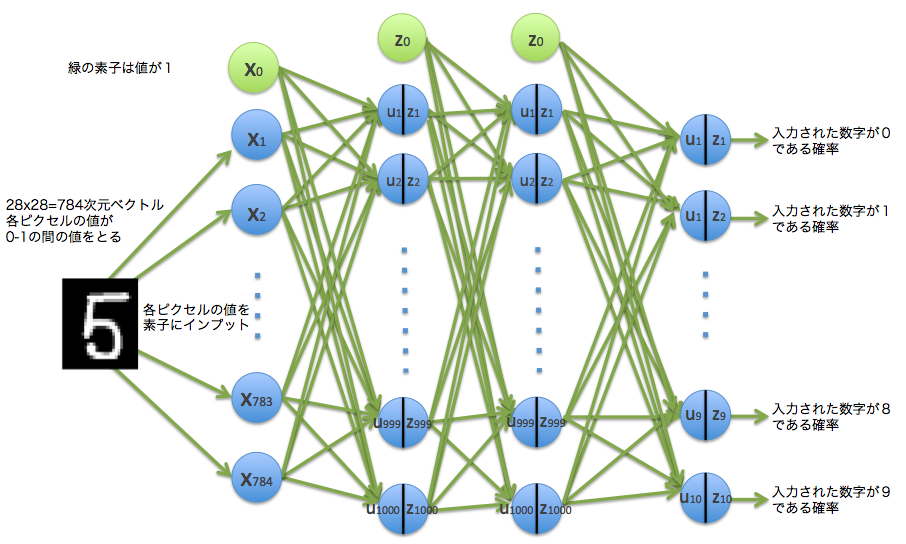
Since the input handwritten digit data is a 784-dimensional vector, there are 784 input elements. This time, the middle layer is specified as 1000 in n_units. The output will be 10 because it identifies the numbers. Below is an image of this model.

The structure of forward propagation is defined by the forward () function below.

# Neural net architecture
#Neural network structure
def forward(x_data, y_data, train=True):
    x, t = Variable(x_data), Variable(y_data)
    h1 = F.dropout(F.relu(model.l1(x)),  train=train)
    h2 = F.dropout(F.relu(model.l2(h1)), train=train)
    y  = model.l3(h2)
    #Since it is a multi-class classification, the softmax function as an error function
    #Derivation of error using cross entropy function
    return F.softmax_cross_entropy(y, t), F.accuracy(y, t)

I would like to explain each function here. In Chainer's method, data is converted from an array to an object of type (class) called Variable of Chainer and used.

x, t = Variable(x_data), Variable(y_data)

The activation function is not the sigmoid function, but the F.relu () function.

F.relu(model.l1(x))

This F.relu () is a Rectified Linear Unit function

f(x) = \max(0, x)

In other words

It is like this. Click here for the drawing code.

# F.relu test
x_data = np.linspace(-10, 10, 100, dtype=np.float32)
x = Variable(x_data)
y = F.relu(x)

plt.figure(figsize=(7,5))
plt.ylim(-2,10)
plt.plot(x.data, y.data)
plt.show()

It's a simple function. For this reason, it seems that the advantage is that the amount of calculation is small and the learning speed is fast.

Next, the F.dropout () function is used with the output of this relu () function as input.

F.dropout(F.relu(model.l1(x)),  train=train)

This dropout function F.dropout () was proposed in the paper Dropout: A Simple Way to Prevent Neural Networks from Overfitting. It seems that overfitting can be prevented by randomly dropping the middle layer (assuming it does not exist) with the method.

Let's move it a little.

# dropout(x, ratio=0.5, train=True)test
# x:Input value
# ratio:Probability of outputting 0
# train:If False, return x as it is
# return:0 with a probability of ratio, with a probability of 1-ratio,x*(1/(1-ratio))Returns the value of

n = 50
v_sum = 0
for i in range(n):
    x_data = np.array([1,2,3,4,5,6], dtype=np.float32)
    x = Variable(x_data)
    dr = F.dropout(x, ratio=0.6,train=True)
    
    for j in range(6):
        sys.stdout.write( str(dr.data[j]) + ', ' )
    print("")
    v_sum += dr.data

#The average of output is x_Approximately matches data
sys.stdout.write( str((v_sum/float(n))) )

output

2.5, 5.0, 7.5, 0.0, 0.0, 0.0, 
2.5, 5.0, 7.5, 10.0, 0.0, 15.0, 
0.0, 5.0, 7.5, 10.0, 12.5, 15.0, 
・ ・ ・
0.0, 0.0, 7.5, 10.0, 0.0, 0.0, 
2.5, 0.0, 7.5, 10.0, 0.0, 15.0, 
[ 0.94999999  2.29999995  3.          3.5999999   7.25        5.69999981]

Pass the array [1,2,3,4,5,6] to the F.dropout () function. Now, ratio is the dropout rate, and since ratio = 0.6 is set, there is a 60% chance that it will be dropped out and 0 will be output. The value is returned with a probability of 40%, but at that time, the probability of returning a value has been reduced to 40%, so to make up for it, $ {1 \ over 0.4} $ times = 2.5 times. The value is output. In other words

(0 \times 0.6 + 2.5 \times 0.4) = 1

So, on average, it is the original number. In the above example, the last line is the average of the output, but it is repeated 50 times and the value is close to the original [1,2,3,4,5,6].

There is another layer of the same structure, and the output value is $ y $.

    h2 = F.dropout(F.relu(model.l2(h1)), train=train)
    y  = model.l3(h2)

The final output is the error output using the softmax function and the cross entropy function. And the precision is returned by the F.accuracy () function.

    #Since it is a multi-class classification, the softmax function as an error function
    #Derivation of error using cross entropy function
    return F.softmax_cross_entropy(y, t), F.accuracy(y, t)

It's a softmax function,

y_k = z_k = f_{k}({\bf u})={\exp(u_{k}) \over \sum_j^K \exp(u_{j})}

By sandwiching this function, the sum of 10 outputs of $ y_1, \ cdots, y_ {10} $ becomes 1, and the outputs can be interpreted as probabilities. I understand that the reason why the $ \ exp () $ function is used is that the value should not be negative.

The familiar $ \ exp () $ function is Since it has a shape like, it does not take a negative value. As a result, the value does not become negative and the sum is 1, which can be interpreted as a probability. Using the output value $ y_k $ of the softmax function, the cross entropy function

E({\bf w}) = -\sum_{n=1}^{N} \sum_{k=1}^{K} t_{nk} \log y_k ({\bf x}_n, {\bf w})

It is expressed as.

In Chainer code, https://github.com/pfnet/chainer/blob/master/chainer/functions/softmax_cross_entropy.py It is in,

def forward_cpu(self, inputs):
        x, t = inputs
        self.y, = Softmax().forward_cpu((x,))
        return -numpy.log(self.y[xrange(len(t)), t]).sum(keepdims=True) / t.size,

Corresponds to.

Also, F.accuracy (y, t) matches the output with the teacher data and returns the correct answer rate.

3.3 Optimizer settings

Now that the model has been decided, let's move on to training. Adam is used here as an optimization method.

# Setup optimizer
optimizer = optimizers.Adam()
optimizer.setup(model.collect_parameters())

Echizen_tm explains Adam in Adam in 30 minutes. I am.

4. Training implementation and results

From the above preparations, we will discriminate handwritten numbers by mini-batch learning and check the accuracy.

train_loss = []
train_acc  = []
test_loss = []
test_acc  = []

l1_W = []
l2_W = []
l3_W = []

# Learning loop
for epoch in xrange(1, n_epoch+1):
    print 'epoch', epoch

    # training
    #Randomly sort the order of N pieces
    perm = np.random.permutation(N)
    sum_accuracy = 0
    sum_loss = 0
    #Learning using data from 0 to N for each batch size
    for i in xrange(0, N, batchsize):
        x_batch = x_train[perm[i:i+batchsize]]
        y_batch = y_train[perm[i:i+batchsize]]

        #Initialize the gradient
        optimizer.zero_grads()
        #Calculate error and accuracy by forward propagation
        loss, acc = forward(x_batch, y_batch)
        #Calculate gradient with error backpropagation
        loss.backward()
        optimizer.update()

        train_loss.append(loss.data)
        train_acc.append(acc.data)
        sum_loss     += float(cuda.to_cpu(loss.data)) * batchsize
        sum_accuracy += float(cuda.to_cpu(acc.data)) * batchsize

    #Display the error of training data and the accuracy of correct answer
    print 'train mean loss={}, accuracy={}'.format(sum_loss / N, sum_accuracy / N)

    # evaluation
    #Check the generalization performance by calculating the error and correct answer accuracy from the test data
    sum_accuracy = 0
    sum_loss     = 0
    for i in xrange(0, N_test, batchsize):
        x_batch = x_test[i:i+batchsize]
        y_batch = y_test[i:i+batchsize]

        #Calculate error and accuracy by forward propagation
        loss, acc = forward(x_batch, y_batch, train=False)

        test_loss.append(loss.data)
        test_acc.append(acc.data)
        sum_loss     += float(cuda.to_cpu(loss.data)) * batchsize
        sum_accuracy += float(cuda.to_cpu(acc.data)) * batchsize

    #Display the error in the test data and the accuracy of the correct answer
    print 'test  mean loss={}, accuracy={}'.format(sum_loss / N_test, sum_accuracy / N_test)

    #Save learned parameters
    l1_W.append(model.l1.W)
    l2_W.append(model.l2.W)
    l3_W.append(model.l3.W)

#Graph drawing accuracy and error
plt.figure(figsize=(8,6))
plt.plot(range(len(train_acc)), train_acc)
plt.plot(range(len(test_acc)), test_acc)
plt.legend(["train_acc","test_acc"],loc=4)
plt.title("Accuracy of digit recognition.")
plt.plot()

Here is the summary result for each epoch. It can be discriminated with high accuracy of about 98.5% by turning 20 times.

output

epoch 1
train mean loss=0.278375425202, accuracy=0.914966667456
test  mean loss=0.11533634907, accuracy=0.964300005436
epoch 2
train mean loss=0.137060894324, accuracy=0.958216670454
test  mean loss=0.0765812527167, accuracy=0.976100009084
epoch 3
train mean loss=0.107826075749, accuracy=0.966816672881
test  mean loss=0.0749603212342, accuracy=0.97770000577
epoch 4
train mean loss=0.0939164237926, accuracy=0.970616674324
test  mean loss=0.0672153823725, accuracy=0.980000005364
epoch 5
train mean loss=0.0831089563683, accuracy=0.973950009048
test  mean loss=0.0705943618687, accuracy=0.980100004673
epoch 6
train mean loss=0.0752325405277, accuracy=0.976883343955
test  mean loss=0.0732760328815, accuracy=0.977900006771
epoch 7
train mean loss=0.0719517664274, accuracy=0.977383343875
test  mean loss=0.063611669606, accuracy=0.981900005937
epoch 8
train mean loss=0.0683009948514, accuracy=0.978566677173
test  mean loss=0.0604036964733, accuracy=0.981400005221
epoch 9
train mean loss=0.0621755663728, accuracy=0.980550010701
test  mean loss=0.0591542539285, accuracy=0.982400006652
epoch 10
train mean loss=0.0618313539471, accuracy=0.981183344225
test  mean loss=0.0693172766063, accuracy=0.982900006175
epoch 11
train mean loss=0.0583098273944, accuracy=0.982000010014
test  mean loss=0.0668152360269, accuracy=0.981600006819
epoch 12
train mean loss=0.054178619228, accuracy=0.983533344865
test  mean loss=0.0614466062452, accuracy=0.982900005579
epoch 13
train mean loss=0.0532431817259, accuracy=0.98390001148
test  mean loss=0.060112986485, accuracy=0.98400000751
epoch 14
train mean loss=0.0538122716064, accuracy=0.983266676267
test  mean loss=0.0624165921964, accuracy=0.983300005198
epoch 15
train mean loss=0.0501562882114, accuracy=0.983833344777
test  mean loss=0.0688113694015, accuracy=0.98310000658
epoch 16
train mean loss=0.0513108611095, accuracy=0.984533343514
test  mean loss=0.0724038232205, accuracy=0.982200007439
epoch 17
train mean loss=0.0471463404785, accuracy=0.985666677058
test  mean loss=0.0612579581685, accuracy=0.983600008488
epoch 18
train mean loss=0.0460166006556, accuracy=0.986050010125
test  mean loss=0.0654888718335, accuracy=0.984400007725
epoch 19
train mean loss=0.0458772557077, accuracy=0.986433342795
test  mean loss=0.0602016936944, accuracy=0.984400007129
epoch 20
train mean loss=0.046333729005, accuracy=0.986433343093
test  mean loss=0.0621869922416, accuracy=0.985100006461

Here is a graph of the discrimination accuracy and error for each batch. The red one is the training data and the blue one is the test data.

Previously, the article [Machine learning] k-nearest neighbor method (k-nearest neighbor method) is written in python by oneself and recognizes handwritten numbers So, I was also trying to distinguish handwritten numbers, but the accuracy at that time was about 97%, so I can see that it has improved a little further.

This Chiner can be operated entirely with Python code, so I think it's a very nice framework for Pythonista. I haven't done "deep" learning yet, it's just a feedforward neural network, so I'd like to write an article about "deep" soon.

5. Matching answers

Let's display the 100 identified numbers. I extracted 100 at random, but the answer is almost correct. After displaying 100 items several times, I was finally able to display one wrong part, so an example is shown below. It feels like humans are being tested (laughs)

(* 4 in 2 rows and 3 columns is misidentified as 9)

plt.style.use('fivethirtyeight')
def draw_digit3(data, n, ans, recog):
    size = 28
    plt.subplot(10, 10, n)
    Z = data.reshape(size,size)   # convert from vector to 28x28 matrix
    Z = Z[::-1,:]             # flip vertical
    plt.xlim(0,27)
    plt.ylim(0,27)
    plt.pcolor(Z)
    plt.title("ans=%d, recog=%d"%(ans,recog), size=8)
    plt.gray()
    plt.tick_params(labelbottom="off")
    plt.tick_params(labelleft="off")
    

plt.figure(figsize=(15,15))

cnt = 0
for idx in np.random.permutation(N)[:100]:
    
    xxx = x_train[idx].astype(np.float32)
    h1 = F.dropout(F.relu(model.l1(Variable(xxx.reshape(1,784)))),  train=False)
    h2 = F.dropout(F.relu(model.l2(h1)), train=False)
    y  = model.l3(h2)
    cnt+=1
    draw_digit3(x_train[idx], cnt, y_train[idx], np.argmax(y.data))
plt.show

6. Visualization of parameter w of the first layer

Input layer parameter $ w ^ {(1)} $ 7 I tried to map and display a dimensional vector as 28x28 pixels. 100 out of 1000 are randomly selected. If you look closely, there are some that look like "2", "5", or "0". You can see the atmosphere that the features can be extracted with the parameters of the first layer.

def draw_digit2(data, n, i):
    size = 28
    plt.subplot(10, 10, n)
    Z = data.reshape(size,size)   # convert from vector to 28x28 matrix
    Z = Z[::-1,:]             # flip vertical
    plt.xlim(0,27)
    plt.ylim(0,27)
    plt.pcolor(Z)
    plt.title("%d"%i, size=9)
    plt.gray()
    plt.tick_params(labelbottom="off")
    plt.tick_params(labelleft="off")

plt.figure(figsize=(10,10))
cnt = 1
for i in np.random.permutation(1000)[:100]:
    draw_digit2(l1_W[len(l1_W)-1][i], cnt, i)
    cnt += 1
    
plt.show()

7. Visualization of output layer parameter w

The output layer is a layer that receives 1000 inputs and outputs 10 outputs, but I also tried to visualize this. The place where "0" is written is the parameter to distinguish the handwritten number as "0".

Since it is a 1000-dimensional vector, 24 0s are added to the end to create a 32x32 image.

#Layer 3
def draw_digit2(data, n, i):
    size = 32
    plt.subplot(4, 4, n)
    data = np.r_[data,np.zeros(24)]
    Z = data.reshape(size,size)   # convert from vector to 28x28 matrix
    Z = Z[::-1,:]             # flip vertical
    plt.xlim(0,size-1)
    plt.ylim(0,size-1)
    plt.pcolor(Z)
    plt.title("%d"%i, size=9)
    plt.gray()
    plt.tick_params(labelbottom="off")
    plt.tick_params(labelleft="off")

plt.figure(figsize=(10,10))
cnt = 1
for i in range(10):
    draw_digit2(l3_W[len(l3_W)-1][i], cnt, i)
    cnt += 1
    
plt.show()

8. Bonus

The number of elements in the intermediate layer was set to [100, 500, 800, 900, 1000, 1100, 1200, 1500, 2000] and each was discriminated. The resulting graph is below. With more than 500 elements, we have achieved about 98%, and it seems that the number of elements beyond that does not change much.

9. Bonus 2: Activation function

For the main activation functions pre-installed in Chainer

• ReLu function
• tanh function
• sigmoid function

there is. It looks like the figure below. It is a function that goes between the input and output of the element, and has the role of setting the threshold value for input and output.

#Activation function test
x_data = np.linspace(-10, 10, 100, dtype=np.float32)
x = Variable(x_data)

y = F.relu(x)
plt.figure(figsize=(8,15))
plt.subplot(311)
plt.title("ReLu function.")
plt.ylim(-2,10)
plt.xlim(-6,6)
plt.plot(x.data, y.data)

y = F.tanh(x)
plt.subplot(312)
plt.title("tanh function.")
plt.ylim(-1.5,1.5)
plt.xlim(-6,6)
plt.plot(x.data, y.data)

y = F.sigmoid(x)
plt.subplot(313)
plt.title("sigmoid function.")
plt.ylim(-.2,1.2)
plt.xlim(-6,6)
plt.plot(x.data, y.data)
plt.show()

Next article "[Deep learning] Try Autoencoder with Chainer to visualize the results." This is an article that implements Autoencoder, a technology that automates feature extraction with deep learning.

[Reference book] Deep Learning (Machine Learning Professional Series) Takayuki Okatani

[Reference website] Chainer's main site 　　　http://chainer.org/ Chainer's GitHub repository 　　　https://github.com/pfnet/chainer Chainer tutorials and references 　　　http://docs.chainer.org/en/latest/ 　"Dropout: A Simple Way to Prevent Neural Networks from Overfitting" 　 Nitish Srivastava, Geoffrey Hinton, Alex Krizhevsky, Ilya Sutskever, Ruslan Salakhutdinov 　　　http://www.cs.toronto.edu/~rsalakhu/papers/srivastava14a.pdf